NLP 3：Interfacing your NLP to Ipopt

Ipopt has been designed to be flexible for a wide variety of applications, and there are a number of ways to interface with Ipopt that allow specific data structures and linear solver techniques.Nevertheless, the authors have included a standard representation that should meet the needs of most users. 

这个教程将讨论6个IPOP接口，分别是 AMPL 建模语言[5]接口，和 C++, C, Fortran, Java, and R 语言接口。 AMPL is a modeling language tool that allows users to write their optimization problem in a syntax that resembles the way the problem would be written mathematically. Once the problem has been formulated in AMPL, the problem can be easily solved using the (already compiled) Ipopt AMPL solver executable, ipopt. Interfacing your problem by directly linking code requires more effort to write, but can be far more efficient for large problems.

We will illustrate how to use each of the four interfaces using an example problem, number 71 from the Hock-Schittkowsky test suite [6],

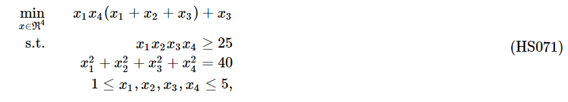
 with the starting point

and the optimal solution

You can find further, less documented examples for using Ipopt from your own source code in the Ipopt/examples subdirectory.

Using Ipopt through AMPL

Using the AMPL solver executable is by far the easiest way to solve a problem with Ipopt. The user must simply formulate the problem in AMPL syntax, and solve the problem through the AMPL environment. There are drawbacks, however. AMPL is a 3rd party package and, as such, must be appropriately licensed (a free student version for limited problem size is available from the AMPL website. Furthermore, the AMPL environment may be prohibitive for very large problems. Nevertheless, formulating the problem in AMPL is straightforward and even for large problems, it is often used as a prototyping tool before using one of the code interfaces.

This tutorial is not intended as a guide to formulating models in AMPL. If you are not already familiar with AMPL, please consult [5].

The problem presented in (HS071) can be solved with Ipopt with the following AMPL model.

# tell ampl to use the ipopt executable as a solver
# make sure ipopt is in the path!
option solver ipopt;

# declare the variables and their bounds, 
# set notation could be used, but this is straightforward
var x1 >= 1, <= 5; 
var x2 >= 1, <= 5; 
var x3 >= 1, <= 5; 
var x4 >= 1, <= 5;

# specify the objective function
minimize obj:
    x1 * x4 * (x1 + x2 + x3) + x3;

# specify the constraints
s.t.
  inequality:
    x1 * x2 * x3 * x4 >= 25;

  equality:
    x1^2 + x2^2 + x3^2 +x4^2 = 40;

# specify the starting point            
let x1 := 1;
let x2 := 5;
let x3 := 5;
let x4 := 1;

# solve the problem
solve;

# print the solution
display x1;
display x2;
display x3;
display x4;

The line, option solver ipopt; tells AMPL to use Ipopt as the solver. The Ipopt executable (installed in Compiling and Installing Ipopt) must be in the PATH for AMPL to find it. The remaining lines specify the problem in AMPL format. The problem can now be solved by starting AMPL and loading the mod file:

$ ampl
> model hs071_ampl.mod;
.
.
.

The problem will be solved using Ipopt and the solution will be displayed.

At this point, AMPL users may wish to skip the sections about interfacing with code, but should read Ipopt Options and Ipopt Output.

Using Ipopt from the command line

It is possible to solve AMPL problems with Ipopt directly from the command line. However, this requires a file in format .nl produced by ampl. If you have a model and data loaded in Ampl, you can create the corresponding .nl file with name, say, myprob.nl by using the Ampl command:

write gmyprob

There is a small .nl file available in the Ipopt distribution. It is located at Ipopt/test/mytoy.nl. We use this file in the remainder of this section. We assume that the file mytoy.nl is in the current directory and that the command ipopt is a shortcut for running the Ipopt binary available in the bin directory of the installation of Ipopt.

We list below commands to perform basic tasks from the Linux prompt.

• To solve mytoy.nl from the Linux prompt, use:

  ipopt mytoy

• To see all command line options for Ipopt, use:

  ipopt -=

• To see more detailed information on all options for Ipopt:

  ipopt mytoy 'print_options_documentation yes'

• To run ipopt, setting the maximum number of iterations to 2 and print level to 4:

  ipopt mytoy 'max_iter 2 print_level 4'

If many options are to be set, they can be collected in a file ipopt.opt that is automatically read by Ipopt, if present, in the current directory, see also Ipopt Options.

Interfacing with Ipopt through code

In order to solve a problem, Ipopt needs more information than just the problem definition (for example, the derivative information). If you are using a modeling language like AMPL, the extra information is provided by the modeling tool and the Ipopt interface. When interfacing with Ipopt through your own code, however, you must provide this additional information. The following information is required by Ipopt:

1. Problem dimensions
   • number of variables
   • number of constraints
2. Problem bounds
   • variable bounds
   • constraint bounds
3. Initial starting point
   • Initial values for the primal x variables
   • Initial values for the multipliers (only required for a warm start option)
4. Problem Structure
   • number of nonzeros in the Jacobian of the constraints
   • number of nonzeros in the Hessian of the Lagrangian function
   • sparsity structure of the Jacobian of the constraints
   • sparsity structure of the Hessian of the Lagrangian function
5. Evaluation of Problem Functions
   Information evaluated using a given point ( x, λ, σf coming from Ipopt)
   • Objective function, f(x)
   • Gradient of the objective, 
     
   • Constraint function values, g(x)
   • Jacobian of the constraints, 
   • Hessian of the Lagrangian function, 
     (this is not required if a quasi-Newton options is chosen to approximate the second derivatives)

The problem dimensions and bounds are straightforward and come solely from the problem definition. The initial starting point is used by the algorithm when it begins iterating to solve the problem. If Ipopt has difficulty converging, or if it converges to a locally infeasible point, adjusting the starting point may help. Depending on the starting point, Ipopt may also converge to different local solutions.

Providing the sparsity structure of derivative matrices is a bit more involved. Ipopt is a nonlinear programming solver that is designed for solving large-scale, sparse problems. While Ipopt can be customized for a variety of matrix formats, the triplet format is used for the standard interfaces in this tutorial. For an overview of the triplet format for sparse matrices, see Triplet Format for Sparse Matrices. Before solving the problem, Ipopt needs to know the number of nonzero elements and the sparsity structure (row and column indices of each of the nonzero entries) of the constraint Jacobian and the Lagrangian function Hessian. Once defined, this nonzero structure MUST remain constant for the entire optimization procedure. This means that the structure needs to include entries for any element that could ever be nonzero, not only those that are nonzero at the starting point.

As Ipopt iterates, it will need the values for problem functions evaluated at particular points. Before we can begin coding the interface, however, we need to work out the details of these equations symbolically for example problem (HS071).

The gradient of the objective f(x) is given by

 and the Jacobian of the constraints g(x) is

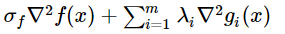
We also need to determine the Hessian of the Lagrangian. (If a quasi-Newton option is chosen to approximate the second derivatives, this is not required. However, if second derivatives can be computed, it is often worthwhile to let Ipopt use them, since the algorithm is then usually more robust and converges faster. More on the quasi-Newton approximation in Quasi-Newton Approximation of Second Derivatives.) The Lagrangian function for the NLP (HS071) is defined as f(x)+g(x)Tλ and the Hessian of the Lagrangian function is, technically, However, we introduce a factor in front of the objective term so that Ipopt can ask for the Hessian of the objective or the constraints independently, if required. Thus, for Ipopt the symbolic form of the Hessian of the Lagrangian is

 

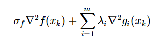
 and for the example problem this becomes

where the first term comes from the Hessian of the objective function, and the second and third term from the Hessian of the constraints. Therefore, the dual variables λ1 and λ2 are the multipliers for the constraints.

The remaining sections of the tutorial will lead you through the coding required to solve example problem (HS071) using, first C++, then C, and finally Fortran. Completed versions of these examples can be found in $IPOPTDIR/Ipopt/examples under hs071_cpp, hs071_c, and hs071_f.

As a user, you are responsible for coding two sections of the program that solves a problem using Ipopt: the main executable (e.g., main) and the problem representation. Typically, you will write an executable that prepares the problem, and then passes control over to Ipopt through an Optimize or Solve call. In this call, you will give Ipopt everything that it requires to call back to your code whenever it needs functions evaluated (like the objective function, the Jacobian of the constraints, etc.). In each of the three sections that follow (C++, C, and Fortran), we will first discuss how to code the problem representation, and then how to code the executable.

The C++ Interface

This tutorial assumes that you are familiar with the C++ programming language, however, we will lead you through each step of the implementation. For the problem representation, we will create a class that inherits off of the pure virtual base class, Ipopt::TNLP. For the executable (the main function) we will make the call to Ipopt through the Ipopt::IpoptApplication class. In addition, we will also be using the Ipopt::SmartPtr class which implements a reference counting pointer that takes care of memory management (object deletion) for you (for details, see The Smart Pointer Implementation: SmartPtr<T>).

After make install (see Compiling and Installing Ipopt), the header files that define these classes are installed in $PREFIX/include/coin-or.

Coding the Problem Representation

We provide the required information by coding the HS071_NLP class, a specific implementation of the TNLP base class. In the executable, we will create an instance of the HS071_NLP class and give this class to Ipopt so it can evaluate the problem functions through the Ipopt::TNLP interface. If you have any difficulty as the implementation proceeds, have a look at the completed example in the Ipopt/examples/hs071_cpp directory.

Start by creating a new directory MyExample under examples and create the files hs071_nlp.hpp and hs071_nlp.cpp. In hs071_nlp.hpp, include IpTNLP.hpp (the base class), tell the compiler that we are using the namespace Ipopt, and create the declaration of the HS071_NLP class, inheriting off of TNLP. Have a look at the Ipopt::TNLP class; you will see eight pure virtual methods that we must implement. Declare these methods in the header file. Implement each of the methods in HS071_NLP.cpp using the descriptions given below. In hs071_nlp.cpp, first include the header file for your class and tell the compiler that you are using the namespace Ipopt. A full version of these files can be found in the Ipopt/examples/hs071_cpp directory.

It is very easy to make mistakes in the implementation of the function evaluation methods, in particular regarding the derivatives. Ipopt has a feature that can help you to debug the derivative code, using finite differences, see Derivative Checker.

Note that the return value of any bool-valued function should be true, unless an error occurred, for example, because the value of a problem function could not be evaluated at the required point.

 Ipopt::TNLP::get_nlp_info

virtual bool get_nlp_info(
      Index&          n,
      Index&          m,
      Index&          nnz_jac_g,
      Index&          nnz_h_lag,
      IndexStyleEnum& index_style
   ) = 0;

Method to request the initial information about the problem. Ipopt uses this information when allocating the arrays that it will later ask you to fill with values. Be careful in this method since incorrect values will cause memory bugs which may be very difficult to find.

 Parameters

n	(out) Storage for the number of variables x
m	(out) Storage for the number of constraints g(x)
nnz_jac_g	(out) Storage for the number of nonzero entries in the Jacobian
nnz_h_lag	(out) Storage for the number of nonzero entries in the Hessian
index_style	(out) Storage for the index style, the numbering style used for row/col entries in the sparse matrix format (TNLP::C_STYLE: 0-based, TNLP::FORTRAN_STYLE: 1-based; see also Triplet Format for Sparse Matrices)

 Our example problem has 4 variables (n), and 2 constraints (m). The constraint Jacobian for this small problem is actually dense and has 8 nonzeros (we still need to represent this Jacobian using the sparse matrix triplet format). The Hessian of the Lagrangian has 10 "symmetric" nonzeros (i.e., nonzeros in the lower left triangular part.). Keep in mind that the number of nonzeros is the total number of elements that may ever be nonzero, not just those that are nonzero at the starting point. This information is set once for the entire problem.

// returns the size of the problem
bool HS071_NLP::get_nlp_info(
   Index&          n,
   Index&          m,
   Index&          nnz_jac_g,
   Index&          nnz_h_lag,
   IndexStyleEnum& index_style
)
{
   // The problem described in HS071_NLP.hpp has 4 variables, x[0] through x[3]
   n = 4;
   // one equality constraint and one inequality constraint
   m = 2;
   // in this example the jacobian is dense and contains 8 nonzeros
   nnz_jac_g = 8;
   // the Hessian is also dense and has 16 total nonzeros, but we
   // only need the lower left corner (since it is symmetric)
   nnz_h_lag = 10;
   // use the C style indexing (0-based)
   index_style = TNLP::C_STYLE;
   return true;
}

Ipopt::TNLP::get_bounds_info

   virtual bool get_bounds_info(
      Index   n,
      Number* x_l,
      Number* x_u,
      Index   m,
      Number* g_l,
      Number* g_u
   ) = 0;

Method to request bounds on the variables and constraints.

Parameters

n	(in) the number of variables x in the problem
x_l	(out) the lower bounds xL for the variables x
x_u	(out) the upper bounds xU for the variables x
m	(in) the number of constraints g(x) in the problem
g_l	(out) the lower bounds gL for the constraints g(x)
g_u	(out) the upper bounds gU for the constraints g(x)

Returns

true if success, false otherwise.

The values of n and m that were specified in TNLP::get_nlp_info are passed here for debug checking. Setting a lower bound to a value less than or equal to the value of the option nlp_lower_bound_inf will cause Ipopt to assume no lower bound. Likewise, specifying the upper bound above or equal to the value of the option nlp_upper_bound_inf will cause Ipopt to assume no upper bound. These options are set to -10¹⁹ and 10¹⁹, respectively, by default, but may be modified by changing these options.

In our example, the first constraint has a lower bound of 25 and no upper bound, so we set the lower bound of constraint to 25 and the upper bound to some number greater than 10¹⁹. The second constraint is an equality constraint and we set both bounds to 40. Ipopt recognizes this as an equality constraint and does not treat it as two inequalities.

// returns the variable bounds
bool HS071_NLP::get_bounds_info(
   Index   n,
   Number* x_l,
   Number* x_u,
   Index   m,
   Number* g_l,
   Number* g_u
)
{
   // here, the n and m we gave IPOPT in get_nlp_info are passed back to us.
   // If desired, we could assert to make sure they are what we think they are.
   assert(n == 4);
   assert(m == 2);
   // the variables have lower bounds of 1
   for( Index i = 0; i < 4; i++ )
   {
      x_l[i] = 1.0;
   }
   // the variables have upper bounds of 5
   for( Index i = 0; i < 4; i++ )
   {
      x_u[i] = 5.0;
   }
   // the first constraint g1 has a lower bound of 25
   g_l[0] = 25;
   // the first constraint g1 has NO upper bound, here we set it to 2e19.
   // Ipopt interprets any number greater than nlp_upper_bound_inf as
   // infinity. The default value of nlp_upper_bound_inf and nlp_lower_bound_inf
   // is 1e19 and can be changed through ipopt options.
   g_u[0] = 2e19;
   // the second constraint g2 is an equality constraint, so we set the
   // upper and lower bound to the same value
   g_l[1] = g_u[1] = 40.0;
   return true;
}

Ipopt::TNLP::get_starting_point

   virtual bool get_starting_point(
      Index   n,
      bool    init_x,
      Number* x,
      bool    init_z,
      Number* z_L,
      Number* z_U,
      Index   m,
      bool    init_lambda,
      Number* lambda
   ) = 0;

Method to request the starting point before iterating.

Parameters

n	(in) the number of variables x in the problem; it will have the same value that was specified in TNLP::get_nlp_info
init_x	(in) if true, this method must provide an initial value for x
x	(out) the initial values for the primal variables x
init_z	(in) if true, this method must provide an initial value for the bound multipliers  and
z_L	(out) the initial values for the bound multipliers
z_U	(out) the initial values for the bound multipliers
m	(in) the number of constraints g(x) in the problem; it will have the same value that was specified in TNLP::get_nlp_info
init_lambda	(in) if true, this method must provide an initial value for the constraint multipliers λ
lambda	(out) the initial values for the constraint multipliers, λ

Returns

true if success, false otherwise.

The boolean variables indicate whether the algorithm requires to have x, z_L/z_u, and lambda initialized, respectively. If, for some reason, the algorithm requires initializations that cannot be provided, false should be returned and Ipopt will stop. The default options only require initial values for the primal variables x.

Note, that the initial values for bound multiplier components for absent bounds are ignored.

In our example, we provide initial values for x as specified in the example problem. We do not provide any initial values for the dual variables, but use an assert to immediately let us know if we are ever asked for them.

// returns the initial point for the problem
bool HS071_NLP::get_starting_point(
   Index   n,
   bool    init_x,
   Number* x,
   bool    init_z,
   Number* z_L,
   Number* z_U,
   Index   m,
   bool    init_lambda,
   Number* lambda
)
{
   // Here, we assume we only have starting values for x, if you code
   // your own NLP, you can provide starting values for the dual variables
   // if you wish
   assert(init_x == true);
   assert(init_z == false);
   assert(init_lambda == false);
   // initialize to the given starting point
   x[0] = 1.0;
   x[1] = 5.0;
   x[2] = 5.0;
   x[3] = 1.0;
   return true;
}

Ipopt::TNLP::eval_f

   virtual bool eval_f(
      Index         n,
      const Number* x,
      bool          new_x,
      Number&       obj_value
   ) = 0;

Method to request the value of the objective function.

Parameters

n	(in) the number of variables x in the problem; it will have the same value that was specified in TNLP::get_nlp_info
x	(in) the values for the primal variables x at which the objective function f(x) is to be evaluated
new_x	(in) false if any evaluation method (eval_*) was previously called with the same values in x, true otherwise. This can be helpful when users have efficient implementations that calculate multiple outputs at once. Ipopt internally caches results from the TNLP and generally, this flag can be ignored.
obj_value	(out) storage for the value of the objective function f(x)

Returns

true if success, false otherwise.

For our example, we ignore the new_x flag and calculate the objective.

// returns the value of the objective function
bool HS071_NLP::eval_f(
   Index         n,
   const Number* x,
   bool          new_x,
   Number&       obj_value
)
{
   assert(n == 4);
   obj_value = x[0] * x[3] * (x[0] + x[1] + x[2]) + x[2];
   return true;
}

Ipopt::TNLP::eval_grad_f

   virtual bool eval_grad_f(
      Index         n,
      const Number* x,
      bool          new_x,
      Number*       grad_f
   ) = 0;

Method to request the gradient of the objective function.

Parameters

n	(in) the number of variables x in the problem; it will have the same value that was specified in TNLP::get_nlp_info
x	(in) the values for the primal variables x at which the gradient ∇f(x) is to be evaluated
new_x	(in) false if any evaluation method (eval_*) was previously called with the same values in x, true otherwise; see also TNLP::eval_f
grad_f	(out) array to store values of the gradient of the objective function ∇f(x). The gradient array is in the same order as the x variables (i.e., the gradient of the objective with respect to x[2] should be put in grad_f[2]).

Returns

true if success, false otherwise.

In our example, we ignore the new_x flag and calculate the values for the gradient of the objective.

// return the gradient of the objective function grad_{x} f(x)
bool HS071_NLP::eval_grad_f(
   Index         n,
   const Number* x,
   bool          new_x,
   Number*       grad_f
)
{
   assert(n == 4);
   grad_f[0] = x[0] * x[3] + x[3] * (x[0] + x[1] + x[2]);
   grad_f[1] = x[0] * x[3];
   grad_f[2] = x[0] * x[3] + 1;
   grad_f[3] = x[0] * (x[0] + x[1] + x[2]);
   return true;
}

Ipopt::TNLP::eval_g

   virtual bool eval_g(
      Index         n,
      const Number* x,
      bool          new_x,
      Index         m,
      Number*       g
   ) = 0;

Method to request the constraint values.

Parameters

n	(in) the number of variables x in the problem; it will have the same value that was specified in TNLP::get_nlp_info
x	(in) the values for the primal variables x at which the constraint functions g(x) are to be evaluated
new_x	(in) false if any evaluation method (eval_*) was previously called with the same values in x, true otherwise; see also TNLP::eval_f
m	(in) the number of constraints g(x) in the problem; it will have the same value that was specified in TNLP::get_nlp_info
g	(out) array to store constraint function values g(x), do not add or subtract the bound values gL or gU.

Returns

true if success, false otherwise.

In our example, we ignore the new_x flag and calculate the values of constraint functions.

// return the value of the constraints: g(x)
bool HS071_NLP::eval_g(
   Index         n,
   const Number* x,
   bool          new_x,
   Index         m,
   Number*       g
)
{
   assert(n == 4);
   assert(m == 2);
   g[0] = x[0] * x[1] * x[2] * x[3];
   g[1] = x[0] * x[0] + x[1] * x[1] + x[2] * x[2] + x[3] * x[3];
   return true;
}

明天继续。。。。