一、图像梯度算法
1、图像梯度-Sobel算子
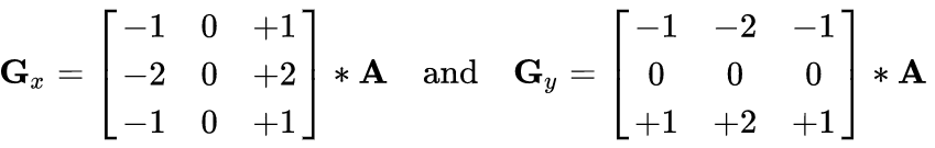
dst = cv2.Sobel(src, ddepth, dx, dy, ksize)
- ddepth:图像的深度
- dx和dy分别表示水平和竖直方向
- ksize是Sobel算子的大小
 1 # *******************图像梯度算法**********************开始
 2 import cv2
 3 # import numpy as np
 4
 5 img = cv2.imread('pie.png',cv2.IMREAD_GRAYSCALE)
 6 cv2.imshow("img",img)
 7 cv2.waitKey()
 8 cv2.destroyAllWindows()
 9
10 # 显示图像函数
11 def cv_show(img,name):
12     cv2.imshow(name,img)
13     cv2.waitKey()
14     cv2.destroyAllWindows()
15
16 # Sobel算子——x轴
17 sobelx = cv2.Sobel(img,cv2.CV_64F,1,0,ksize=3)   # 计算水平的
18 cv_show(sobelx,'sobelx')
19
20 # 白到黑是正数,黑到白就是负数了,所有的负数会被截断成0,所以要取绝对值
21 sobelx = cv2.Sobel(img,cv2.CV_64F,1,0,ksize=3)
22 sobelx = cv2.convertScaleAbs(sobelx)             # 取绝对值
23 cv_show(sobelx,'sobelx')
24
25 # Sobel算子——y轴
26 sobely = cv2.Sobel(img,cv2.CV_64F,0,1,ksize=3)
27 sobely = cv2.convertScaleAbs(sobely)             # 取绝对值
28 cv_show(sobely,'sobely')
29
30 # 求和
31 sobelxy = cv2.addWeighted(sobelx,0.5,sobely,0.5,0)  # 按权重计算
32 cv_show(sobelxy,'sobelxy')
33
34 # 也有直接计算xy轴的————不推荐使用
35 # sobelxy=cv2.Sobel(img,cv2.CV_64F,1,1,ksize=3)
36 # sobelxy = cv2.convertScaleAbs(sobelxy)
37 # cv_show(sobelxy,'sobelxy')
38 # *******************图像梯度算法**********************结束
用lena图像来实际操作一下:
 1 # *******************图像梯度算法-实际操作**********************开始
 2 import cv2
 3
 4 # 显示图像函数
 5 def cv_show(img,name):
 6     cv2.imshow(name,img)
 7     cv2.waitKey()
 8     cv2.destroyAllWindows()
 9
10 img = cv2.imread('lena.jpg',cv2.IMREAD_GRAYSCALE)
11 cv_show(img,'img')
12
13 # 分别计算x和y
14 img = cv2.imread('lena.jpg',cv2.IMREAD_GRAYSCALE)
15 sobelx = cv2.Sobel(img,cv2.CV_64F,1,0,ksize=3)
16 sobelx = cv2.convertScaleAbs(sobelx)
17 sobely = cv2.Sobel(img,cv2.CV_64F,0,1,ksize=3)
18 sobely = cv2.convertScaleAbs(sobely)
19 sobelxy = cv2.addWeighted(sobelx,0.5,sobely,0.5,0)
20 cv_show(sobelxy,'sobelxy')
21 # *******************图像梯度算法-实际操作**********************结束


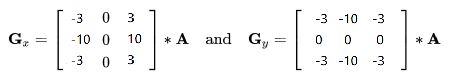
2、图像梯度-Scharr和Laplacian算子
(1)Scharr算子
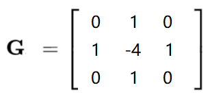
(2)Laplacian算子
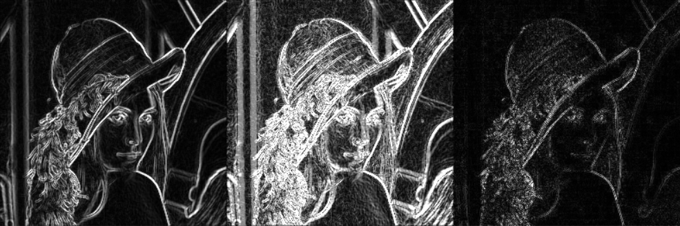
(3)不同算子之间的差距
 1 # *******************图像梯度算子-Scharr+laplacian**********************开始
 2 import cv2
 3 import numpy as np
 4
 5 #不同算子的差异
 6 img = cv2.imread('lena.jpg',cv2.IMREAD_GRAYSCALE)
 7 sobelx = cv2.Sobel(img,cv2.CV_64F,1,0,ksize=3)
 8 sobely = cv2.Sobel(img,cv2.CV_64F,0,1,ksize=3)
 9 sobelx = cv2.convertScaleAbs(sobelx)
10 sobely = cv2.convertScaleAbs(sobely)
11 sobelxy =  cv2.addWeighted(sobelx,0.5,sobely,0.5,0)
12
13 scharrx = cv2.Scharr(img,cv2.CV_64F,1,0)
14 scharry = cv2.Scharr(img,cv2.CV_64F,0,1)
15 scharrx = cv2.convertScaleAbs(scharrx)
16 scharry = cv2.convertScaleAbs(scharry)
17 scharrxy =  cv2.addWeighted(scharrx,0.5,scharry,0.5,0)
18
19 laplacian = cv2.Laplacian(img,cv2.CV_64F)
20 laplacian = cv2.convertScaleAbs(laplacian)
21
22 res = np.hstack((sobelxy,scharrxy,laplacian))
23
24 # 显示图像函数
25 def cv_show(img,name):
26     cv2.imshow(name,img)
27     cv2.waitKey()
28     cv2.destroyAllWindows()
29 cv_show(res,'res')
30 # *******************图像梯度算子-Scharr+laplacian**********************结束
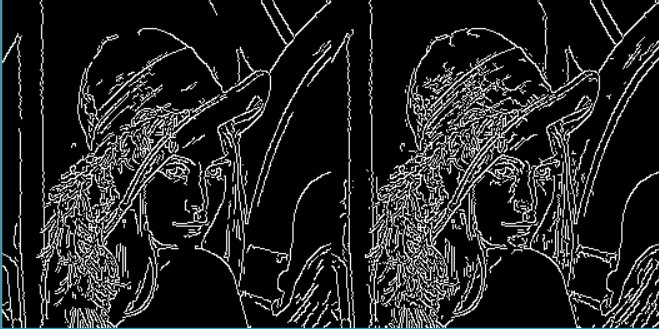
二、边缘检测
Canny边缘检测
-
1) 使用高斯滤波器,以平滑图像,滤除噪声。
-
2) 计算图像中每个像素点的梯度强度和方向。
-
3) 应用非极大值(Non-Maximum Suppression)抑制,以消除边缘检测带来的杂散响应。
-
4) 应用双阈值(Double-Threshold)检测来确定真实的和潜在的边缘。
-
5) 通过抑制孤立的弱边缘最终完成边缘检测。
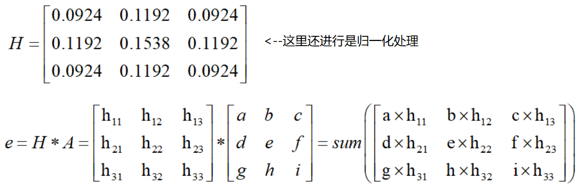
1、高斯滤波器
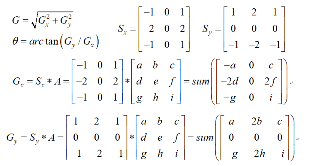
2、梯度和方向
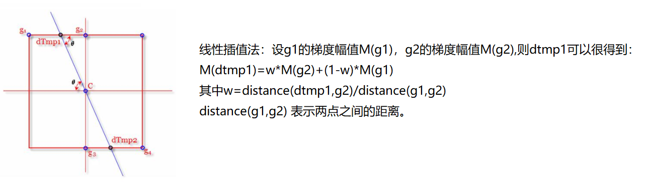
3、非极大值抑制

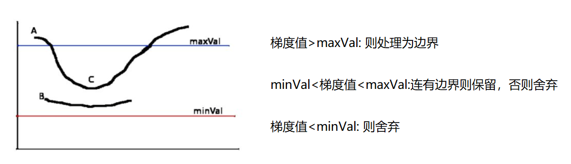
4、双阈值检测
 1 # *******************边缘检测**********************开始
 2 import cv2
 3 import numpy as np
 4
 5 img=cv2.imread("lena.jpg",cv2.IMREAD_GRAYSCALE)
 6
 7 v1=cv2.Canny(img,80,150)  # 设置双阈值 最小和最大
 8 v2=cv2.Canny(img,50,100)
 9
10 res = np.hstack((v1,v2))
11
12 # 显示图像函数
13 def cv_show(img,name):
14     cv2.imshow(name,img)
15     cv2.waitKey()
16     cv2.destroyAllWindows()
17 cv_show(res,'res')
18 # *******************边缘检测**********************结束
三、图像金字塔
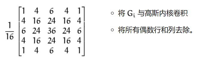
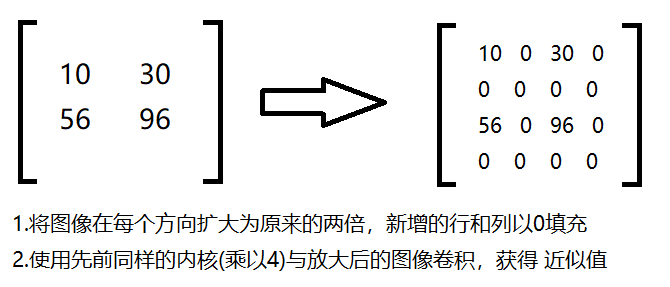
1、高斯金字塔
(1)高斯金字塔:向下采样方法(缩小)
(2)高斯金字塔:向上采样方法(放大)
 1 # *******************图像金字塔--高斯金字塔**********************开始
 2 import cv2
 3 import numpy as np
 4
 5 # 显示图像函数
 6 def cv_show(img,name):
 7     cv2.imshow(name,img)
 8     cv2.waitKey()
 9     cv2.destroyAllWindows()
10
11 img=cv2.imread("AM.png")
12 # cv_show(img,'img')
13 print (img.shape)
14
15 # 高斯金字塔-上采样 (可执行多次)
16 up=cv2.pyrUp(img)
17 # cv_show(up,'up')
18 print (up.shape)
19
20 # 高斯金字塔-下采样 (可执行多次)
21 down=cv2.pyrDown(img)
22 # cv_show(down,'down')
23 print (down.shape)
24
25 # 高斯金字塔-先上采样再下采样 (会损失信息-变模糊)
26 up=cv2.pyrUp(img)
27 up_down=cv2.pyrDown(up)
28 # cv_show(up_down,'up_down')
29 cv_show(np.hstack((img,up_down)),'up_down')
30 # *******************图像金字塔--高斯金字塔**********************结束

2、拉普拉斯金字塔
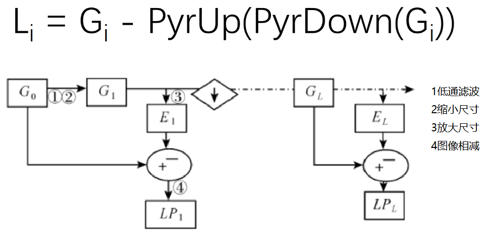
 1 # *******************图像金字塔-拉普拉斯金字塔**********************开始
 2 import cv2
 3 import numpy as np
 4
 5 # 显示图像函数
 6 def cv_show(img,name):
 7     cv2.imshow(name,img)
 8     cv2.waitKey()
 9     cv2.destroyAllWindows()
10
11 img=cv2.imread("AM.png")
12 down=cv2.pyrDown(img)
13 down_up=cv2.pyrUp(down)
14 l_1=img-down_up
15 cv_show(l_1,'l_1')
16 # *******************图像金字塔-拉普拉斯金字塔**********************结束
四、图像轮廓
cv2.findContours(img,mode,method)
mode:轮廓检索模式
- RETR_EXTERNAL :只检索最外面的轮廓;
- RETR_LIST:检索所有的轮廓,并将其保存到一条链表当中;
- RETR_CCOMP:检索所有的轮廓,并将他们组织为两层:顶层是各部分的外部边界,第二层是空洞的边界;
- RETR_TREE:检索所有的轮廓,并重构嵌套轮廓的整个层次;
method:轮廓逼近方法
- CHAIN_APPROX_NONE:以Freeman链码的方式输出轮廓,所有其他方法输出多边形(顶点的序列)。
- CHAIN_APPROX_SIMPLE:压缩水平的、垂直的和斜的部分,也就是,函数只保留他们的终点部分。
为提高准确性,使用二值图像。
1、轮廓检测及绘制
 1 # *******************图像轮廓**********************开始
 2 import cv2
 3 import numpy as np
 4
 5 # 读入图像转换为二值图像
 6 img = cv2.imread('contours.png')
 7 gray = cv2.cvtColor(img, cv2.COLOR_BGR2GRAY)     # 转换为灰度图
 8 ret, thresh = cv2.threshold(gray, 127, 255, cv2.THRESH_BINARY)  # 转换成二值图
 9
10 # 显示图像函数
11 def cv_show(img,name):
12     cv2.imshow(name,img)
13     cv2.waitKey()
14     cv2.destroyAllWindows()
15 # cv_show(thresh,'thresh')
16
17 # 轮廓检测  第一个就是二值的结果  第二个是一堆轮廓点  第三个是层级
18 binary, contours, hierarchy = cv2.findContours(thresh, cv2.RETR_TREE, cv2.CHAIN_APPROX_NONE)
19
20 # 绘制轮廓
21 draw_img = img.copy()  # 注意需要copy,要不原图会变。。。
22 res = cv2.drawContours(draw_img, contours, -1, (0, 0, 255), 2) # 传入绘制图像,轮廓,轮廓索引(-1全部),颜色模式,线条厚度
23 # cv_show(res,'res')
24
25 draw_img = img.copy()
26 res = cv2.drawContours(draw_img, contours, 2, (0, 0, 255), 2)
27 cv_show(res,'res')
28 # *******************图像轮廓**********************结束

2、轮廓特征
 1 import cv2
 2
 3 # 读入图像转换为二值图像
 4 img = cv2.imread('contours.png')
 5 gray = cv2.cvtColor(img, cv2.COLOR_BGR2GRAY)     # 转换为灰度图
 6 ret, thresh = cv2.threshold(gray, 127, 255, cv2.THRESH_BINARY)  # 转换成二值图
 7
 8 # 轮廓检测  第一个就是二值的结果  第二个是一堆轮廓点  第三个是层级
 9 binary, contours, hierarchy = cv2.findContours(thresh, cv2.RETR_TREE, cv2.CHAIN_APPROX_NONE)
10
11 # 绘制轮廓
12 draw_img = img.copy()
13 res = cv2.drawContours(draw_img, contours, 2, (0, 0, 255), 2)
14
15 # 轮廓特征
16 cnt = contours[0]               # 获取轮廓
17 print(cv2.contourArea(cnt))     # 计算面积
18 print(cv2.arcLength(cnt, True)) # 计算周长,True表示闭合的
3、轮廓近似

 1 import cv2
 2
 3 img = cv2.imread('contours2.png')
 4 # 显示图像函数
 5 def cv_show(img,name):
 6     cv2.imshow(name,img)
 7     cv2.waitKey()
 8     cv2.destroyAllWindows()
 9
10 # 二值+轮廓检测
11 gray = cv2.cvtColor(img, cv2.COLOR_BGR2GRAY)
12 ret, thresh = cv2.threshold(gray, 127, 255, cv2.THRESH_BINARY)
13 binary, contours, hierarchy = cv2.findContours(thresh, cv2.RETR_TREE, cv2.CHAIN_APPROX_NONE)
14 cnt = contours[0]
15 # 轮廓绘制
16 draw_img = img.copy()
17 res = cv2.drawContours(draw_img, [cnt], -1, (0, 0, 255), 2)
18 # cv_show(res,'res')
19
20 # 轮廓近似
21 epsilon = 0.05*cv2.arcLength(cnt,True)
22 approx = cv2.approxPolyDP(cnt,epsilon,True)
23
24 draw_img = img.copy()
25 res = cv2.drawContours(draw_img, [approx], -1, (0, 0, 255), 2)
26 cv_show(res,'res')

(1)边界矩形
 1 # *******************图像轮廓-边界矩形**********************开始
 2 import cv2
 3
 4 # 显示图像函数
 5 def cv_show(img,name):
 6     cv2.imshow(name,img)
 7     cv2.waitKey()
 8     cv2.destroyAllWindows()
 9
10 img = cv2.imread('contours.png')
11
12 gray = cv2.cvtColor(img, cv2.COLOR_BGR2GRAY)
13 ret, thresh = cv2.threshold(gray, 127, 255, cv2.THRESH_BINARY)
14 binary, contours, hierarchy = cv2.findContours(thresh, cv2.RETR_TREE, cv2.CHAIN_APPROX_NONE)
15 cnt = contours[0]
16
17 # 边界矩形
18 x,y,w,h = cv2.boundingRect(cnt)
19 img = cv2.rectangle(img,(x,y),(x+w,y+h),(0,255,0),2)
20 cv_show(img,'img')
21 # 轮廓面积与边界矩形比
22 area = cv2.contourArea(cnt)
23 x, y, w, h = cv2.boundingRect(cnt)
24 rect_area = w * h
25 extent = float(area) / rect_area
26 print ('轮廓面积与边界矩形比',extent)
27 # *******************图像轮廓-边界矩形**********************结束
(2)外接圆
1 # 外接圆
2 (x,y),radius = cv2.minEnclosingCircle(cnt)
3 center = (int(x),int(y))
4 radius = int(radius)
5 img = cv2.circle(img,center,radius,(0,255,0),2)
6 cv_show(img,'img')
五、傅里叶变换
https://zhuanlan.zhihu.com/p/19763358
1、傅里叶的作用
-
高频:变化剧烈的灰度分量,例如边界
-
低频:变化缓慢的灰度分量,例如一片大海
2、滤波
-
低通滤波器:只保留低频,会使得图像模糊
-
高通滤波器:只保留高频,会使得图像细节增强
opencv中主要就是cv2.dft()和cv2.idft(),输入图像需要先转换成np.float32 格式,得到的结果中频率为0的部分会在左上角,通常要转换到中心位置,通过shift变换。
3、傅里叶变换
 1 # *******************傅里叶变换**********************开始
 2 import numpy as np
 3 import cv2
 4 from matplotlib import pyplot as plt
 5
 6 img = cv2.imread('lena.jpg',0)
 7
 8 img_float32 = np.float32(img)
 9
10 # 傅里叶变换
11 dft = cv2.dft(img_float32, flags = cv2.DFT_COMPLEX_OUTPUT)
12 dft_shift = np.fft.fftshift(dft)                            # 低频值移动到中间
13
14 # 对两通道进行转换——映射公式
15 magnitude_spectrum = 20*np.log(cv2.magnitude(dft_shift[:,:,0],dft_shift[:,:,1]))
16
17 plt.subplot(121),plt.imshow(img, cmap = 'gray')
18 plt.title('Input Image'), plt.xticks([]), plt.yticks([])
19 plt.subplot(122),plt.imshow(magnitude_spectrum, cmap = 'gray')
20 plt.title('Magnitude Spectrum'), plt.xticks([]), plt.yticks([])
21 plt.show()
22 # *******************傅里叶变换**********************结束

4、高通、低通滤波器
低通滤波器:
 1 # *******************低通滤波器**********************开始
 2 import numpy as np
 3 import cv2
 4 from matplotlib import pyplot as plt
 5
 6 img = cv2.imread('lena.jpg',0)
 7
 8 img_float32 = np.float32(img)
 9
10 # 傅里叶变换
11 dft = cv2.dft(img_float32, flags = cv2.DFT_COMPLEX_OUTPUT)
12 dft_shift = np.fft.fftshift(dft)
13
14 rows, cols = img.shape
15 crow, ccol = int(rows/2) , int(cols/2)     # 中心位置
16
17 # 低通滤波
18 mask = np.zeros((rows, cols, 2), np.uint8)  # 掩码
19 mask[crow-30:crow+30, ccol-30:ccol+30] = 1  # 区域
20
21 # IDFT
22 fshift = dft_shift*mask                     # 掩码结合
23 f_ishift = np.fft.ifftshift(fshift)         # 位置还原
24 img_back = cv2.idft(f_ishift)               # 傅里叶逆变换
25 img_back = cv2.magnitude(img_back[:,:,0],img_back[:,:,1]) # 图像转换
26
27 plt.subplot(121),plt.imshow(img, cmap = 'gray')
28 plt.title('Input Image'), plt.xticks([]), plt.yticks([])
29 plt.subplot(122),plt.imshow(img_back, cmap = 'gray')
30 plt.title('Result'), plt.xticks([]), plt.yticks([])
31
32 plt.show()
33 # *******************低通滤波器**********************结束

高通滤波器:
 1 # *******************高通滤波器**********************开始
 2 import numpy as np
 3 import cv2
 4 from matplotlib import pyplot as plt
 5
 6 img = cv2.imread('lena.jpg',0)
 7
 8 img_float32 = np.float32(img)
 9
10 dft = cv2.dft(img_float32, flags = cv2.DFT_COMPLEX_OUTPUT)
11 dft_shift = np.fft.fftshift(dft)
12
13 rows, cols = img.shape
14 crow, ccol = int(rows/2) , int(cols/2)     # 中心位置
15
16 # 高通滤波
17 mask = np.ones((rows, cols, 2), np.uint8)  # 掩码
18 mask[crow-30:crow+30, ccol-30:ccol+30] = 0
19
20 # IDFT
21 fshift = dft_shift*mask
22 f_ishift = np.fft.ifftshift(fshift)
23 img_back = cv2.idft(f_ishift)
24 img_back = cv2.magnitude(img_back[:,:,0],img_back[:,:,1])
25
26 plt.subplot(121),plt.imshow(img, cmap = 'gray')
27 plt.title('Input Image'), plt.xticks([]), plt.yticks([])
28 plt.subplot(122),plt.imshow(img_back, cmap = 'gray')
29 plt.title('Result'), plt.xticks([]), plt.yticks([])
30
31 plt.show()
32 # *******************高通滤波器**********************结束
