线性回归小结

根据输入输出变量的不同类型，对预测任务给予不同的名称：输入变量与输出变量均为连续变量的预测问题称为回归问题，输出变量为有限个离散变量的预测问题称为分类问题，输入变量与输出变量均为变量序列的预测问题称为标注问题。这里对线性回归的原理 算法和代码实现做一个小结。

1 线性回归的原理

回归用于预测输入变量和输出变量之间的关系，特别是当输入变量的值发生变化时，输出变量的值随之发生的变化。回归模型是表示从输入变量到输出变量之间映射的函数，回归问题的学习等价于函数拟合：选择一条函数曲线使其很好地拟合已知数据且很好地预测未知数据。
给定数据集(left { left ( x_{1},y_{1}),(x_{2},y_{2},cdot cdot cdot ,(x_{m},y_{m} ight ) ight })，其中(x_{i}=left ( x_{i1};x_{i2};cdot cdot cdot ;x_{in} ight ))，线性回归试图学得一个线性模型以尽可能准确地预测实值输出标记(y_{x})。对应的线性回归模型：
(h_{ heta }left ( x_{1}, x_{2},cdot cdot cdot x_{n} ight )= heta _{0}+ heta _{1}x_{1}+cdot cdot cdot + heta _{n}x_{n})，其中( heta _{i}left ( i=0,1,cdot cdot cdot ,n ight ))表示模型参数，(x_{i}left ( i=0,1,cdot cdot cdot ,n ight ))表示每个样本的(n)个特征，令(x_{0}=1)，对应模型简化为:(h_{ heta }left ( x_{1},x_{2},cdot cdot cdot ,x_{n} ight )=sum_{i=0}^{n} heta _{i}x_{i})，其矩阵形式为：$${\mathit{h}}_{\theta }\left(\mathit{X}\right)=\mathit{X}\theta$$
其中，假设函数(h_{ heta }left ( X ight ))是(m imes 1)的向量 $$\theta =\text{[}{\theta }_0{\theta }_1\cdot \cdot \cdot {\theta }_{\mathit{n}}{\text{]}}^{\mathit{T}}$$
$$\mathit{X}=\left(\begin{array}{ccccc}{\mathit{x}}_{11}& {\mathit{x}}_{12}& \cdots & {\mathit{x}}_{1\mathit{n}}& 1\\ {\mathit{x}}_{21}& {\mathit{x}}_{22}& \cdots & {\mathit{x}}_{2\mathit{n}}& 1\\ ⋮& ⋮& \ddots & ⋮& ⋮\\ {\mathit{x}}_{\mathit{m}1}& {\mathit{x}}_{\mathit{m}2}& \cdots & {\mathit{x}}_{\mathit{m}\mathit{n}}& 1\end{array}\right)$$其中，m代表样本个数，n代表样本的特征数。

其模型对应的损失函数：

[Jleft ( heta _{0} , heta _{1},cdots , heta _{n} ight )=sum_{i=1}^{m}left ( h_{ heta }left (x_{0}^{(i)},x_{1}^{(i)},cdots,x_{n}^{(i)} ight ) -y_{i} ight )^{2} ]

损失函数的矩阵形式：

[Jleft ( heta ight )=frac{1}{2}left ( X heta -Y ight )^{T}left ( X heta -Y ight ) ]

线性回归的优化目标：

[min_{ heta _{0}, heta _{2},cdots , heta _{n}}Jleft ( heta _{0}, heta _{2},cdots , heta _{n} ight ) ]

2 线性回归算法

由上一小节的优化目标来看，线性回归的目标是求得一组( heta)参数使损失函数最小。常用的方法有梯度下降法和最小二乘法。

2.1 梯度下降法最小化(Jleft ( heta ight ))

[ heta = heta -alpha frac{partial Jleft ( heta ight )}{partial heta }= heta -alpha X^{T}left ( X heta -Y ight ) ]

2.2 最小二乘法最小化(Jleft ( heta ight ))

[ heta =left ( X^{T} X ight )^{-1}X^{T}Y ]

3 线性回归的代码实现

3.1用线性回归找到最佳拟合直线

标准回归函数和数据导入函数

#regression.py
from numpy import *

def loadDataSet(fileName):
    numFeat = len(open(fileName).readline().split('	')) - 1
    dataMat = []; labelMat = []
    fr = open(fileName)
    for line in fr.readlines():
        lineArr = []
        curLine = line.strip().split('	')
        for i in range(numFeat):
            lineArr.append(float(curLine[i]))
        dataMat.append(lineArr)
        labelMat.append(float(curLine[-1]))
    return dataMat,labelMat

def standRegres(xArr,yArr):
    xMat = mat(xArr); yMat = mat(yArr).T
    xTx = xMat.T*xMat
    if linalg.det(xTx) == 0.0:  #判断行列式是否为0
        print("This matrix is singular, cannot do inverse.")
        return
    ws = xTx.I*(xMat.T*yMat)
    return ws

#实际效果
>>> import regression
>>> import imp
>>> imp.reload(regression)
<module 'regression' from 'D:\Python\Mechine_learning\Regression\regression.py'>
>>> xArr,yArr=regression.loadDataSet('ex0.txt')
>>> xArr[0:2]
[[1.0, 0.067732], [1.0, 0.42781]]
>>> ws=regression.standRegres(xArr,yArr)
>>> ws
matrix([[3.00774324],
        [1.69532264]])

>>> from numpy import *
>>> imp.reload(regression)
<module 'regression' from 'D:\Python\Mechine_learning\Regression\regression.py'>
>>> xMat=mat(xArr)
>>> yMat=mat(yArr)
>>> yHat=xMat*ws
#绘出数据集散点图和最佳拟合直线图
>>> import matplotlib.pyplot as plt
>>> fig = plt.figure()
>>> ax=fig.add_subplot(111)
>>> ax.scatter(xMat[:,1].flatten().A[0],yMat.T[:,0].flatten().A[0])
<matplotlib.collections.PathCollection object at 0x00000276F5B0C550>
>>> xCopy=xMat.copy()
>>> xCopy.sort(0)
>>> yHat=xCopy*ws
>>> ax.plot(xCopy[:,1],yHat)
[<matplotlib.lines.Line2D object at 0x00000276F5B0CE10>]
>>> plt.show()

通过命令corrcoef(yEstimate,yActual)来计算预测值和真实值的相关性，首先计算出y的预测值yMat，再来计算相关系数（这时需要将yMat转置，以保证两个向量都是行向量）。

>>> yHat=xMat*ws
>>> corrcoef(yHat.T, yMat)
array([[1.        , 0.98647356],
       [0.98647356, 1.        ]])

矩阵包含所有两两组合的相关系数。可以看到，对角线上的数据是1.0，因为yMat和自己的匹配是最完美的，而YHat和yMat的相关系数为0.98。

3.2 局部加权线性回归

线性回归的一个问题是有可能出现欠拟合现象，因为它求的是具有最小均方误差的无偏估计。有些方法允许在估计中引入一些偏差，从而降低预测的均方误差。其中的一个方法是局部加权线性回归（Locally Weighted Linear Regression，LWLR）。在该算法中，给待预测点附近的每个点赋予一定的权重，在这个子集上基于最小均方差来进行普通的回归

#局部加权线性回归函数
def lwlr(testPoint,xArr,yArr,k=1.0):
    xMat = mat(xArr); yMat = mat(yArr).T
    m = shape(xMat)[0]
    weights = mat(eye((m))) #创建对角矩阵
    for j in range(m):  #权重值以指数级衰减
        diffMat = testPoint - xMat[j,:]
        weights[j,j] = exp(diffMat*diffMat.T/(-2.0*k**2)) #LWLR用高斯核给待测试点附近的每个点赋予权重
    xTx = xMat.T*(weights*xMat)
    if linalg.det(xTx) == 0.0:
        print("This matrix is singular, cannot do inverse")
        return
    ws = xTx.I*(xMat.T*(weights*yMat))
    return testPoint*ws

def lwlrTest(testArr,xArr,yArr,k=1.0):
    m = shape(testArr)[0]
    yHat = zeros(m)
    for i in range(m):
        yHat[i] = lwlr(testArr[i],xArr,yArr,k)
    return yHat

>>> imp.reload(regression)
<module 'regression' from 'D:\Python\Mechine_learning\Regression\regression.py'>
>>> xArr,yArr=regression.loadDataSet('ex0.txt')
#对单点估计
>>> yArr[0]
3.176513
>>> regression.lwlr(xArr[0],xArr,yArr,1.0)
matrix([[3.12204471]])
>>> regression.lwlr(xArr[0],xArr,yArr,0.001)
matrix([[3.20175729]])

#调用lwlrTest()得到数据集里所有点的估计
>>> yHat=regression.lwlrTest(xArr,xArr,yArr,0.003)

#绘出估计值和原始值 观察yHat的拟合效果
>>> xMat=mat(xArr)
>>> srtInd=xMat[:,1].argsort(0)
>>> xSort=xMat[srtInd][:,0,:]
>>> import matplotlib.pyplot as plt
>>> fig=plt.figure()
>>> ax=fig.add_subplot(111)
>>> ax.plot(xSort[:,1],yHat[srtInd])
[<matplotlib.lines.Line2D object at 0x00000276F558DE80>]
>>> ax.scatter(xMat[:,1].flatten().A[0],mat(yArr).T.flatten().A[0],s=2,c='red')
<matplotlib.collections.PathCollection object at 0x00000276F56D6780>
>>> plt.show()

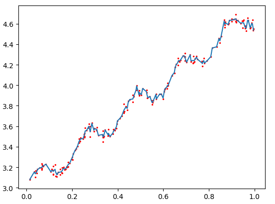
k=0.003

>>> yHat=regression.lwlrTest(xArr,xArr,yArr,0.01)
>>> xMat=mat(xArr)
>>> xSort=xMat[srtInd][:,0,:]
>>> import matplotlib.pyplot as plt
>>> fig=plt.figure()
>>> ax=fig.add_subplot(111)
>>> ax.plot(xSort[:,1],yHat[srtInd])
[<matplotlib.lines.Line2D object at 0x00000276F99BD668>]
>>> ax.scatter(xMat[:,1].flatten().A[0],mat(yArr).T.flatten().A[0],s=2,c='red')
<matplotlib.collections.PathCollection object at 0x00000276F99BDF28>
>>> plt.show()

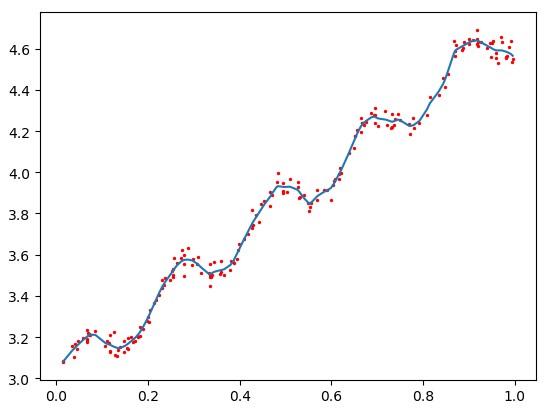
k=0.01

>>> yHat=regression.lwlrTest(xArr,xArr,yArr,1.0)
>>> xMat=mat(xArr)
>>> xSort=xMat[srtInd][:,0,:]
>>> import matplotlib.pyplot as plt
>>> fig=plt.figure()
>>> ax=fig.add_subplot(111)
>>> ax.plot(xSort[:,1],yHat[srtInd])
[<matplotlib.lines.Line2D object at 0x00000276F9B89B00>]
>>> ax.scatter(xMat[:,1].flatten().A[0],mat(yArr).T.flatten().A[0],s=2,c='red')
<matplotlib.collections.PathCollection object at 0x00000276F9B91400>
>>> plt.show()

k=1.0

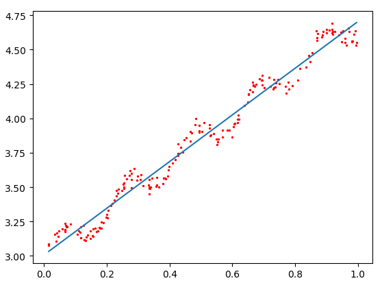
使用3种不同平滑值绘出的局部加权线性回归结果。可以看到，k = 1.0时的模型效果与最小二乘法差不多，k = 0.01时该模型可以挖出数据的潜在规律，而k = 0.003时则考虑了太多的噪声，进而导致了过拟合现象。

=~休息十分钟 再继续吧~=

4 线性回归的示例：预测鲍鱼的年龄

def rssError(yArr,yHatArr):
    return ((yArr-yHatArr)**2).sum()

>>> imp.reload(regression)
<module 'regression' from 'D:\Python\Mechine_learning\Regression\regression.py'>
>>> abX,abY=regression.loadDataSet('abalone.txt')
>>> yHat01=regression.lwlrTest(abX[0:99],abX[0:99],abY[0:99],0.1)
>>> yHat1=regression.lwlrTest(abX[0:99],abX[0:99],abY[0:99],1)
>>> yHat10=regression.lwlrTest(abX[0:99],abX[0:99],abY[0:99],10)
>>> regression.rssError(abY[0:99],yHat01.T)
56.78868743050092
>>> regression.rssError(abY[0:99],yHat1.T)
429.89056187038
>>> regression.rssError(abY[0:99],yHat10.T)
549.1181708827924

使用较小的核将得到较低的误差。那么，为什么不在所有数据集上都使用最小的核呢？这是因为使用最小的核将造成过拟合，对新数据不一定能达到最好的预测效果。下面就来看看它们在新数据上的表现：

>>> yHat01=regression.lwlrTest(abX[100:199],abX[0:99],abY[0:99],0.1)
>>> regression.rssError(abY[100:199],yHat01.T)
57913.51550155911
>>> yHat1=regression.lwlrTest(abX[100:199],abX[0:99],abY[0:99],1)
>>> regression.rssError(abY[100:199],yHat1.T)
573.5261441895982
>>> yHat10=regression.lwlrTest(abX[100:199],abX[0:99],abY[0:99],10)
>>> regression.rssError(abY[100:199],yHat10.T)
517.5711905381903

从上述结果可以看到，在上面的三个参数中，核大小等于10时的测试误差最小，但它在训练集上的误差却是最大的。接下来再来和简单的线性回归做个比较

>>> ws=regression.standRegres(abX[0:99],abY[0:99])
>>> yHat=mat(abX[100:199])*ws
>>> regression.rssError(abY[100:199],yHat.T.A)
518.6363153245542

简单线性回归达到了与局部加权线性回归类似的效果。这也表明一点，必须在未知数据上比较效果才能选取到最佳模型本例展示了如何使用局部加权线性回归来构建模型，可以得到比普通线性回归更好的效果。局部加权线性回归的问题在于，每次必须在整个数据集上运行。也就是说为了做出预测，必须保存所有的训练数据。下面将介绍另一种提高预测精度的方法。

如果数据的特征比样本点还多应该怎么办？是否还可以使用线性回归和之前的方法来做预测？答案是否定的，即不能再使用前面介绍的方法。这是因为在计算((left ( X^{T} X ight )^{-1})的时候会出错。
如果特征比样本点还多（n > m），也就是说输入数据的矩阵X不是满秩矩阵。非满秩矩阵在求逆时会出现问题。为了解决这个问题，统计学家引入了岭回归（ridge regression）的概念，这就是本节将介绍的第一种缩减方法。第二种缩减方法，称为前向逐步回归。

岭回归

#岭回归
def ridgeRegres(xMat, yMat, lam=0.2):  #给定lambda下 计算回归系数
    xTx = xMat.T*xMat
    denom = xTx+eye(shape(xMat)[1])*lam
    if linalg.det(denom) == 0.0:
        print("This matrix is singular, cannot do inverse")
        return
    ws = denom.I*(xMat.T*yMat)
    return ws

def ridgeTest(xArr, yArr):  #用于在一组λ上测试结果
    xMat = mat(xArr); yMat = mat(yArr).T
    yMean = mean(yMat,0)
    yMat = yMat - yMean
    xMeans = mean(xMat,0)
    xVar = var(xMat, 0)
    xMat = (xMat - xMeans)/xVar   #所有特征减去各自的均值并除方差
    numTestPts = 30
    wMat = zeros((numTestPts,shape(xMat)[1]))
    for i in range(numTestPts):  #在30个不同的lambda下调用ridgeRegres() 这里lambda以指数级变化
        ws = ridgeRegres(xMat, yMat, exp(i-10))
        wMat[i,:]=ws.T
    return wMat #所有的回归系数输出到一个矩阵并返回

看一下鲍鱼数据集上的运行结果

>>> imp.reload(regression)
<module 'regression' from 'D:\Python\Mechine_learning\Regression\regression.py'>
>>> abX,abY=regression.loadDataSet('abalone.txt')
>>> ridgeWeights=regression.ridgeTest(abX,abY)
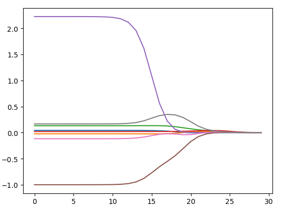
#得到了30个不同lambda所对应的回归系数 绘出了回归系数与log(λ)的关系
>>> import matplotlib.pyplot as plt
>>> fig=plt.figure()
>>> ax=fig.add_subplot(111)
>>> ax.plot(ridgeWeights)
[<matplotlib.lines.Line2D object at 0x00000276FE84D4A8>, <matplotlib.lines.Line2D object at 0x00000276FE84D668>, <matplotlib.lines.Line2D object at 0x00000276FE84D828>, <matplotlib.lines.Line2D object at 0x00000276FE84DA20>, <matplotlib.lines.Line2D object at 0x00000276FE84DC18>, <matplotlib.lines.Line2D object at 0x00000276FE84DE10>, <matplotlib.lines.Line2D object at 0x00000276FE84DFD0>, <matplotlib.lines.Line2D object at 0x00000276FB3F8240>]
>>> plt.show()

前向逐步回归

#标准化
def regularize(xMat):
    inMat = xMat.copy()
    inMeans = mean(inMat,0)
    inVar = var(inMat,0)
    inMat = (inMat - inMeans)/inVar
    return inMat

#前向逐步线性回归
def stageWise(xArr,yArr,eps=0.01,numIt=100):
    """

    :param xArr: 输入数据
    :param yArr: 预测变量
    :param eps: 每次迭代需要调整的步长
    :param numIt: 迭代次数
    :return:
    """
    xMat = mat(xArr); yMat = mat(yArr).T #数据转换并存入矩阵
    yMean = mean(yMat,0)
    yMat = yMat - yMean
    xMat = regularize(xMat) #特征按照均值为0方差为1进行标准化处理
    m,n = shape(xMat)
    returnMat = zeros((numIt,n))
    ws = zeros((n,1)); wsTest = ws.copy(); wsMax = ws.copy() #初始化ws 所有权重设为1 为实现贪心算法建立ws的两个副本
    for i in range(numIt):
        print(ws.T)
        lowestError = inf
        for j in range(n): #遍历所有特征
            for sign in [-1,1]:
                wsTest = ws.copy()
                wsTest[j] += eps*sign #对每个权重增加或减少一个很小的值 得到一个新的W
                yTest = xMat*wsTest  #用于计算增加或减少该特征对误差的影响
                rssE = rssError(yMat.A,yTest.A)  #计算新W下的平方误差
                if rssE < lowestError:
                    lowestError = rssE
                    wsMax = wsTest
        ws = wsMax.copy()
        returnMat[i,:]= ws.T
    return returnMat

>>> imp.reload(regression)
<module 'regression' from 'D:\Python\Mechine_learning\Regression\regression.py'>
>>> xArr,yArr=regression.loadDataSet('abalone.txt')
>>> regression.stageWise(xArr,yArr,0.01,200)
[[0. 0. 0. 0. 0. 0. 0. 0.]]
[[0.   0.   0.   0.01 0.   0.   0.   0.  ]]
[[0.   0.   0.   0.02 0.   0.   0.   0.  ]]
[[0.   0.   0.   0.03 0.   0.   0.   0.  ]]
[[0.   0.   0.   0.04 0.   0.   0.   0.  ]]
[[0.   0.   0.   0.05 0.   0.   0.   0.  ]]
[[0.   0.   0.   0.06 0.   0.   0.   0.  ]]
[[0.   0.   0.01 0.06 0.   0.   0.   0.  ]]
[[0.   0.   0.01 0.06 0.   0.   0.   0.01]]
[[0.   0.   0.01 0.06 0.   0.   0.   0.02]]
[[0.   0.   0.01 0.06 0.   0.   0.   0.03]]
[[0.   0.   0.01 0.06 0.   0.   0.   0.04]]
[[0.   0.   0.01 0.06 0.   0.   0.   0.05]]
[[0.   0.   0.01 0.06 0.   0.   0.   0.06]]
[[0.   0.   0.01 0.06 0.   0.   0.   0.07]]
[[0.   0.   0.01 0.06 0.   0.   0.   0.08]]
[[0.   0.   0.01 0.05 0.   0.   0.   0.08]]
[[0.   0.   0.01 0.05 0.   0.   0.   0.09]]
[[0.   0.   0.01 0.05 0.   0.   0.   0.1 ]]
[[0.   0.   0.01 0.05 0.   0.   0.   0.11]]
[[ 0.    0.    0.01  0.05  0.   -0.01  0.    0.11]]
[[ 0.    0.    0.01  0.05  0.   -0.02  0.    0.11]]
[[ 0.    0.    0.01  0.05  0.   -0.02  0.    0.12]]
[[ 0.    0.    0.01  0.05  0.   -0.03  0.    0.12]]
.
.
.
[[ 0.05  0.    0.09  0.03  0.31 -0.64  0.    0.36]]
[[ 0.04  0.    0.09  0.03  0.31 -0.64  0.    0.36]]
[[ 0.05  0.    0.09  0.03  0.31 -0.64  0.    0.36]]
[[ 0.04  0.    0.09  0.03  0.31 -0.64  0.    0.36]]
[[ 0.05  0.    0.09  0.03  0.31 -0.64  0.    0.36]]
[[ 0.04  0.    0.09  0.03  0.31 -0.64  0.    0.36]]
[[ 0.05  0.    0.09  0.03  0.31 -0.64  0.    0.36]]
[[ 0.04  0.    0.09  0.03  0.31 -0.64  0.    0.36]]
[[ 0.05  0.    0.09  0.03  0.31 -0.64  0.    0.36]]
[[ 0.04  0.    0.09  0.03  0.31 -0.64  0.    0.36]]
[[ 0.05  0.    0.09  0.03  0.31 -0.64  0.    0.36]]
[[ 0.04  0.    0.09  0.03  0.31 -0.64  0.    0.36]]
[[ 0.05  0.    0.09  0.03  0.31 -0.64  0.    0.36]]
[[ 0.04  0.    0.09  0.03  0.31 -0.64  0.    0.36]]
[[ 0.05  0.    0.09  0.03  0.31 -0.64  0.    0.36]]
[[ 0.04  0.    0.09  0.03  0.31 -0.64  0.    0.36]]
[[ 0.05  0.    0.09  0.03  0.31 -0.64  0.    0.36]]
[[ 0.04  0.    0.09  0.03  0.31 -0.64  0.    0.36]]
[[ 0.05  0.    0.09  0.03  0.31 -0.64  0.    0.36]]
[[ 0.04  0.    0.09  0.03  0.31 -0.64  0.    0.36]]

array([[ 0.  ,  0.  ,  0.  , ...,  0.  ,  0.  ,  0.  ],
       [ 0.  ,  0.  ,  0.  , ...,  0.  ,  0.  ,  0.  ],
       [ 0.  ,  0.  ,  0.  , ...,  0.  ,  0.  ,  0.  ],
       ...,
       [ 0.05,  0.  ,  0.09, ..., -0.64,  0.  ,  0.36],
       [ 0.04,  0.  ,  0.09, ..., -0.64,  0.  ,  0.36],
       [ 0.05,  0.  ,  0.09, ..., -0.64,  0.  ,  0.36]])

上述结果中值得注意的是w1和w6都是0，这表明它们不对目标值造成任何影响，也就是说这些特征很可能是不需要的。另外，在参数eps设置为0.01的情况下，一段时间后系数就已经饱和并在特定值之间来回震荡，这是因为步长太大的缘故。这里会看到，第一个权重在0.04和0.05之间来回震荡。
下面试着用更小的步长和更多的步数：

>>> regression.stageWise(xArr,yArr,0.001,5000)
array([[ 0.   ,  0.   ,  0.   , ...,  0.   ,  0.   ,  0.   ],
       [ 0.   ,  0.   ,  0.   , ...,  0.   ,  0.   ,  0.   ],
       [ 0.   ,  0.   ,  0.   , ...,  0.   ,  0.   ,  0.   ],
       ...,
       [ 0.043, -0.011,  0.12 , ..., -0.963, -0.105,  0.187],
       [ 0.044, -0.011,  0.12 , ..., -0.963, -0.105,  0.187],
       [ 0.043, -0.011,  0.12 , ..., -0.963, -0.105,  0.187]])

把这些结果与最小二乘法进行比较，后者的结果可以通过如下代码获得

>>> from numpy import *
>>> imp.reload(regression)
<module 'regression' from 'D:\Python\Mechine_learning\Regression\regression.py'>
>>> xMat=mat(xArr)
>>> yMat=mat(yArr).T
>>> xMat=regression.regularize(xMat)
>>> yM=mean(yMat,0)
>>> yMat=yMat-yM
>>> weights=regression.standRegres(xMat,yMat.T)
>>> weights.T
matrix([[ 0.0430442 , -0.02274163,  0.13214087,  0.02075182,  2.22403814,
         -0.99895312, -0.11725427,  0.16622915]])

可以看到在5000次迭代以后，逐步线性回归算法与常规的最小二乘法效果类似.使用0.005的epsilon值并经过1000次迭代后的结果：

>>> imp.reload(regression)
<module 'regression' from 'D:\Python\Mechine_learning\Regression\regression.py'>
>>> xArr,yArr=regression.loadDataSet('abalone.txt')
>>> ws=regression.stageWise(xArr,yArr,0.005,1000)
>>> import matplotlib.pyplot as plt
>>> fig=plt.figure()
>>> ax=fig.add_subplot(111)
>>> ax.plot(ws)
[<matplotlib.lines.Line2D object at 0x000001B1FDD164A8>, <matplotlib.lines.Line2D object at 0x000001B1FDD16668>, <matplotlib.lines.Line2D object at 0x000001B1FDD16828>, <matplotlib.lines.Line2D object at 0x000001B1FDD16A20>, <matplotlib.lines.Line2D object at 0x000001B1FDD16C18>, <matplotlib.lines.Line2D object at 0x000001B1FDD16E10>, <matplotlib.lines.Line2D object at 0x000001B1FDD16FD0>, <matplotlib.lines.Line2D object at 0x000001B1FDD23240>]
>>> plt.show()

5 线性回归总结

优点：结果易于理解，计算上不复杂。
缺点：对非线性的数据拟合不好。