机器学习算法整理（七）支持向量机以及SMO算法实现

以下均为自己看视频做的笔记，自用，侵删！

还参考了：http://www.ai-start.com/ml2014/

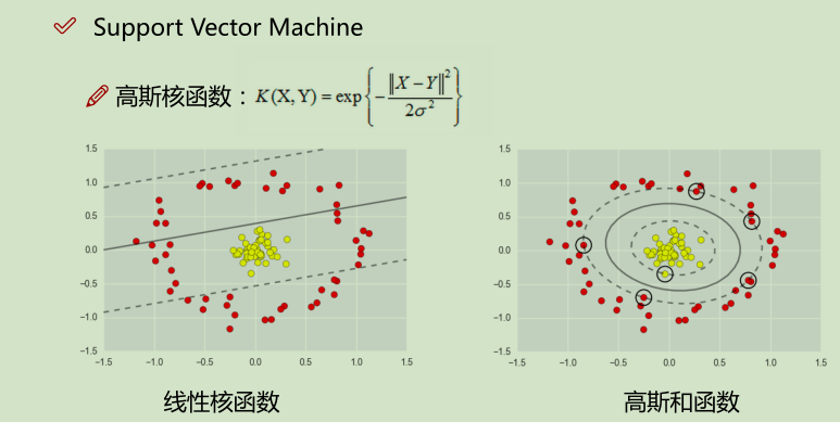
在监督学习中，许多学习算法的性能都非常类似，因此，重要的不是你该选择使用学习算法A还是学习算法B，而更重要的是，应用这些算法时，所创建的大量数据在应用这些算法时，表现情况通常依赖于你的水平。比如：你为学习算法所设计的特征量的选择，以及如何选择正则化参数，诸如此类的事。还有一个更加强大的算法广泛的应用于工业界和学术界，它被称为支持向量机(Support Vector Machine)。与逻辑回归和神经网络相比，支持向量机，或者简称SVM，在学习复杂的非线性方程时提供了一种更为清晰，更加强大的方式。

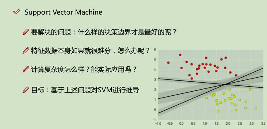
容错能力越强越好

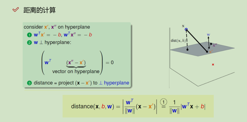
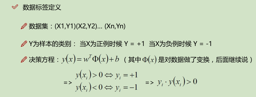
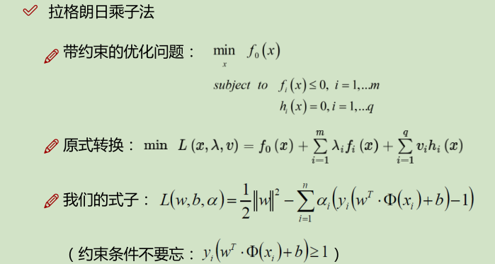
b为平面的偏正向，w为平面的法向量，x到平面的映射：

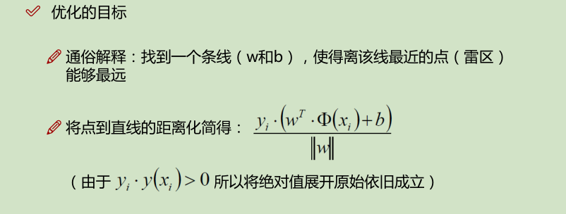
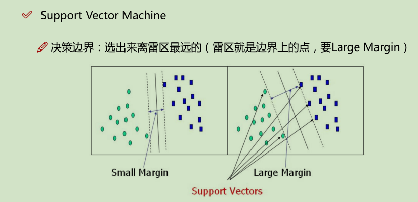
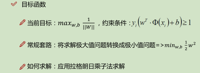
先求的是，距分界线距离最小的点；然后再求的是 什么样的w和b，使得这样的点，距离分界线的值最大。

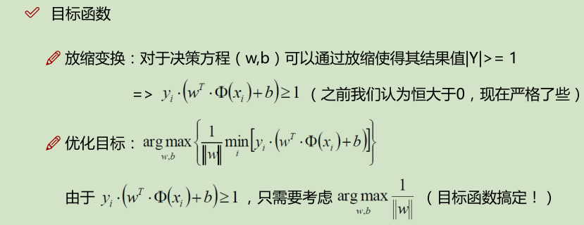
放缩之后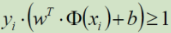：; 又要取 其为min，即 取 yi*(w^T*Q(xi) + b) = 1  => 

补充：

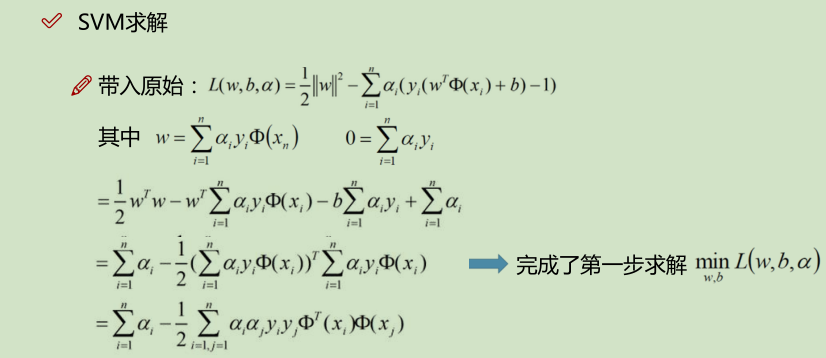
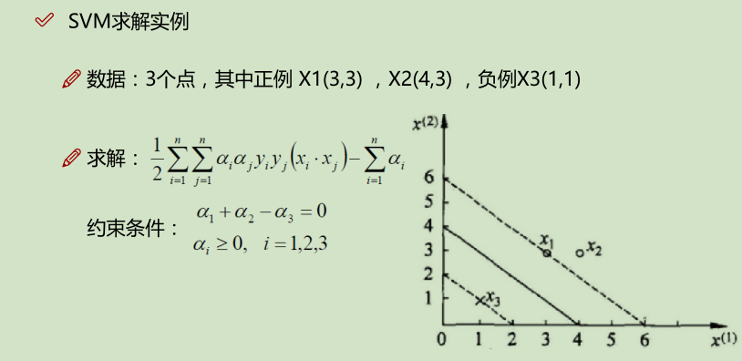
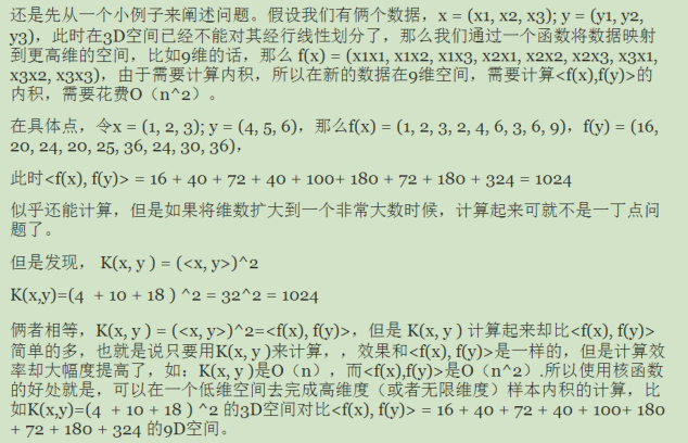
下面的 x_i · x_j   是算的内积：如，(3_i, 3_i) · (3_j, 3_j) ==> 3_i * 3_j + 3_i * 3_j = 18;

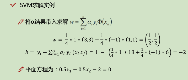
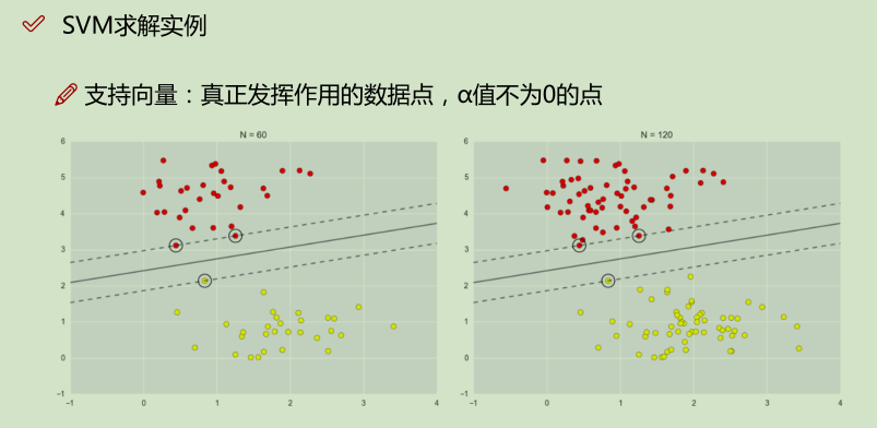
如上面实例，x2就是没有发挥作用的数据点，α为0；x1, x2就是支持向量，α不为0的点；

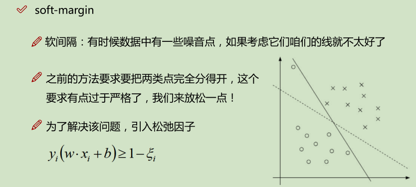
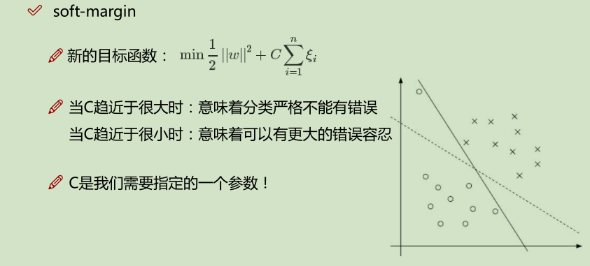
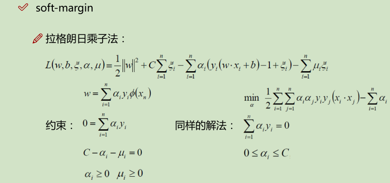
松弛因子：

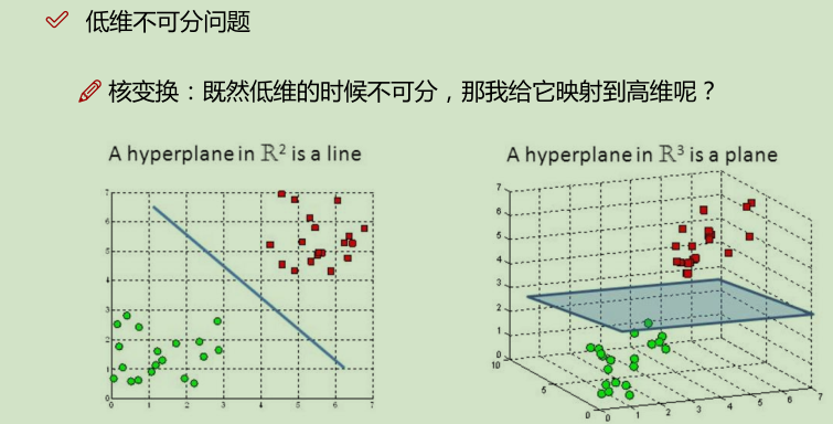
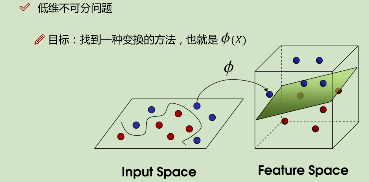
核变换：低微不可分==> 映射到高维

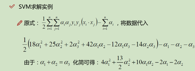
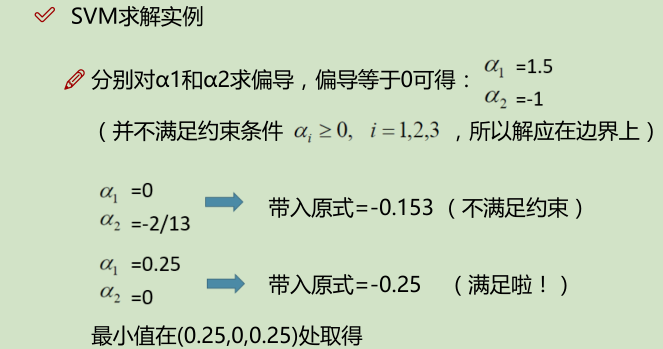
举例：

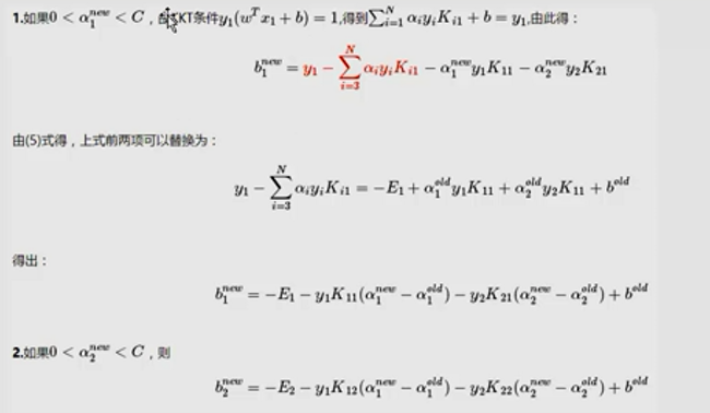
SMO算法实现：

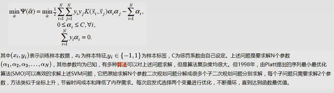
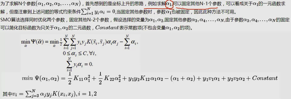
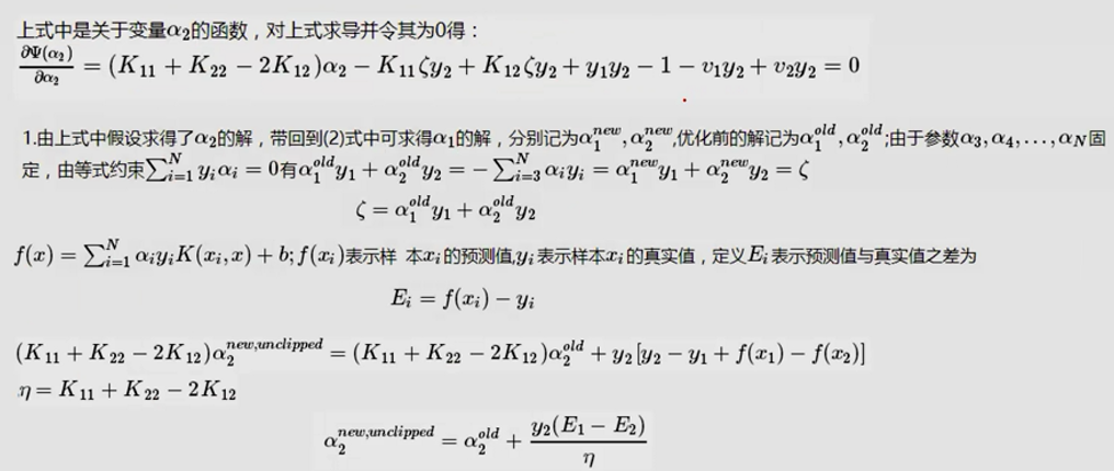
除了α1，α2当成变量，其他的α都当成常数项。

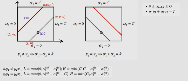
（L是取值的下界，H是取值的上界）

代码实现：

import numpy as np

def loadDataSet(fileName):

    dataMat = []; labelMat = []

    fr = open(fileName)

    for line in fr.readlines():

        lineArr = line.strip().split('	')

        dataMat.append([float(lineArr[0]), float(lineArr[1])])

        labelMat.append(float(lineArr[2]))

    return dataMat,labelMat



def selectJrand(i,m):

    j=i #we want to select any J not equal to i

    while (j==i):

        j = int(np.random.uniform(0,m))

    return j


# 控制aj的上下界
def clipAlpha(aj,H,L):

    if aj > H: 

        aj = H

    if L > aj:

        aj = L

    return aj


# dataMat: 数据; classLabels: Y值; C:V值; toler:容忍程度; maxIter: 最大迭代次数
def smoSimple(dataMatIn, classLabels, C, toler, maxIter):

    #初始化操作
    dataMatrix = np.mat(dataMatIn); labelMat = np.mat(classLabels).transpose()

    b = 0; m,n = np.shape(dataMatrix)

    # 进行初始化
    alphas = np.mat(np.zeros((m,1)))

    iter = 0

    while (iter < maxIter):

        alphaPairsChanged = 0

        # m : 数据样本数
        for i in range(m):
            
            # 先计算FXi，这里只用了线性的 kernel，相当于不变。
            fXi = float(np.multiply(alphas,labelMat).T*(dataMatrix*dataMatrix[i,:].T)) + b

            Ei = fXi - float(labelMat[i])#if checks if an example violates KKT conditions

            # 设置限制条件
            if ((labelMat[i]*Ei < -toler) and (alphas[i] < C)) or ((labelMat[i]*Ei > toler) and (alphas[i] > 0)):

                #随机再选一个不等于i的数
                j = selectJrand(i,m)

                fXj = float(np.multiply(alphas,labelMat).T*(dataMatrix*dataMatrix[j,:].T)) + b

                Ej = fXj - float(labelMat[j])

                alphaIold = alphas[i].copy(); alphaJold = alphas[j].copy();

                # 控制边界条件
                # 定义了上(H)下(L)界取值范围
                if (labelMat[i] != labelMat[j]):

                    L = max(0, alphas[j] - alphas[i])

                    H = min(C, C + alphas[j] - alphas[i])

                else:

                    L = max(0, alphas[j] + alphas[i] - C)

                    H = min(C, alphas[j] + alphas[i])

                if L==H: print "L==H"; continue

                #算出 eta = K11 + K22 - K12
                #这里需要添加一个负号
                eta = 2.0 * dataMatrix[i,:]*dataMatrix[j,:].T - dataMatrix[i,:]*dataMatrix[i,:].T - dataMatrix[j,:]*dataMatrix[j,:].T

                if eta >= 0: print "eta>=0"; continue

                # 即这里就用一个减号
                alphas[j] -= labelMat[j]*(Ei - Ej)/eta

                # 控制上下界
                alphas[j] = clipAlpha(alphas[j],H,L)

                if (abs(alphas[j] - alphaJold) < 0.00001): print "j not moving enough"; continue

                # 算出αi
                alphas[i] += labelMat[j]*labelMat[i]*(alphaJold - alphas[j])#update i by the same amount as j

                                                                        #the update is in the oppostie direction

                b1 = b - Ei- labelMat[i]*(alphas[i]-alphaIold)*dataMatrix[i,:]*dataMatrix[i,:].T - labelMat[j]*(alphas[j]-alphaJold)*dataMatrix[i,:]*dataMatrix[j,:].T

                b2 = b - Ej- labelMat[i]*(alphas[i]-alphaIold)*dataMatrix[i,:]*dataMatrix[j,:].T - labelMat[j]*(alphas[j]-alphaJold)*dataMatrix[j,:]*dataMatrix[j,:].T

                if (0 < alphas[i]) and (C > alphas[i]): b = b1

                elif (0 < alphas[j]) and (C > alphas[j]): b = b2

                else: b = (b1 + b2)/2.0

                alphaPairsChanged += 1

                print "iter: %d i:%d, pairs changed %d" % (iter,i,alphaPairsChanged)

        if (alphaPairsChanged == 0): iter += 1

        else: iter = 0

        print "iteration number: %d" % iter

    return b,alphas

if __name__ == '__main__':
    dataMat,labelMat = loadDataSet('testSet.txt')
    b,alphas = smoSimple(dataMat, labelMat, 0.06, 0.01, 100)
    print 'b:',b
    print 'alphas',alphas[alphas>0]

SMO实例：

import matplotlib.pyplot as plt
import numpy as np
%matplotlib inline
from matplotlib.colors import ListedColormap

def plot_decision_regions(X, y, classifier, test_idx=None, resolution=0.02):
    # setup marker generator and color map
    markers = ('s', 'x', 'o', '^', 'v')
    colors = ('red', 'blue', 'lightgreen', 'gray', 'cyan')
    cmap = ListedColormap(colors[:len(np.unique(y))])
    # plot the decision surface
    x1_min, x1_max = X[:, 0].min() - 1, X[:, 0].max() + 1
    x2_min, x2_max = X[:, 1].min() - 1, X[:, 1].max() + 1
    xx1, xx2 = np.meshgrid(np.arange(x1_min, x1_max, resolution), np.arange(x2_min, x2_max, resolution))
    Z = classifier.predict(np.array([xx1.ravel(), xx2.ravel()]).T)
    Z = Z.reshape(xx1.shape)
    plt.contourf(xx1, xx2, Z, alpha=0.4, cmap=cmap)
    plt.xlim(xx1.min(), xx1.max())
    plt.ylim(xx2.min(), xx2.max())
    # plot class samples
    for idx, cl in enumerate(np.unique(y)):
        plt.scatter(x=X[y == cl, 0], y=X[y == cl, 1],alpha=0.8, c=cmap(idx),marker=markers[idx], label=cl)
    # highlight test samples
    if test_idx:
        X_test, y_test = X[test_idx, :], y[test_idx]
        plt.scatter(X_test[:, 0], X_test[:, 1], c='', alpha=1.0, linewidth=1, marker='o', s=55, label='test set')

from sklearn import datasets
import numpy as np
from sklearn.cross_validation import train_test_split

iris = datasets.load_iris() # 由于Iris是很有名的数据集，scikit-learn已经原生自带了。
X = iris.data[:, [1, 2]]
y = iris.target # 标签已经转换成0，1，2了
X_train, X_test, y_train, y_test = train_test_split(X, y, test_size=0.3, random_state=0) # 为了看模型在没有见过数据集上的表现，随机拿出数据集中30%的部分做测试

# 为了追求机器学习和最优化算法的最佳性能，我们将特征缩放
from sklearn.preprocessing import StandardScaler
sc = StandardScaler()
sc.fit(X_train) # 估算每个特征的平均值和标准差
sc.mean_ # 查看特征的平均值，由于Iris我们只用了两个特征，所以结果是array([ 3.82857143,  1.22666667])
sc.scale_ # 查看特征的标准差，这个结果是array([ 1.79595918,  0.77769705])
X_train_std = sc.transform(X_train)
# 注意：这里我们要用同样的参数来标准化测试集，使得测试集和训练集之间有可比性
X_test_std = sc.transform(X_test)
X_combined_std = np.vstack((X_train_std, X_test_std))
y_combined = np.hstack((y_train, y_test))

# 导入SVC
from sklearn.svm import SVC
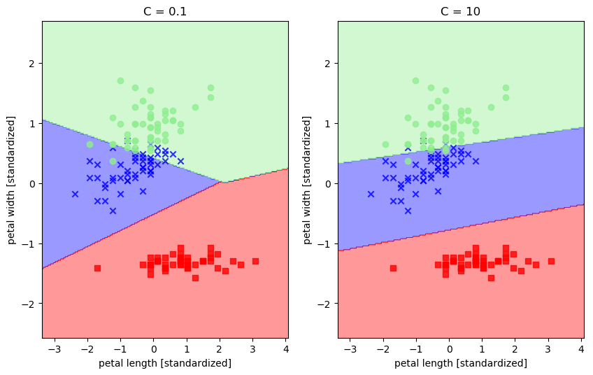
svm1 = SVC(kernel='linear', C=0.1, random_state=0) # 用线性核
svm1.fit(X_train_std, y_train)

svm2 = SVC(kernel='linear', C=10, random_state=0) # 用线性核
svm2.fit(X_train_std, y_train)


fig = plt.figure(figsize=(10,6))
ax1 = fig.add_subplot(1,2,1)
#ax2 = fig.add_subplot(1,2,2)

plot_decision_regions(X_combined_std, y_combined, classifier=svm1)
plt.xlabel('petal length [standardized]')
plt.ylabel('petal width [standardized]')
plt.title('C = 0.1')


ax2 = fig.add_subplot(1,2,2)
plot_decision_regions(X_combined_std, y_combined, classifier=svm2)
plt.xlabel('petal length [standardized]')
plt.ylabel('petal width [standardized]')
plt.title('C = 10')

plt.show()

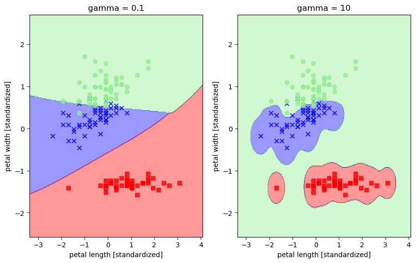
svm1 = SVC(kernel='rbf', random_state=0, gamma=0.1, C=1.0) # 令gamma参数中的x分别等于0.1和10
svm1.fit(X_train_std, y_train) 

svm2 = SVC(kernel='rbf', random_state=0, gamma=10, C=1.0) 
svm2.fit(X_train_std, y_train) 

fig = plt.figure(figsize=(10,6))
ax1 = fig.add_subplot(1,2,1)


plot_decision_regions(X_combined_std, y_combined, classifier=svm1)
plt.xlabel('petal length [standardized]')
plt.ylabel('petal width [standardized]')
plt.title('gamma = 0.1')


ax2 = fig.add_subplot(1,2,2)
plot_decision_regions(X_combined_std, y_combined, classifier=svm2)
plt.xlabel('petal length [standardized]')
plt.ylabel('petal width [standardized]')
plt.title('gamma = 10')

plt.show()