改善深层神经网络-week3编程题（TensorFlow实现手势数字识别）

TensorFlow常用函数

import math
import numpy as np
import h5py
import matplotlib.pyplot as plt
import tensorflow as tf
from tensorflow.python.framework import ops
from tf_utils import load_dataset, random_mini_batches, convert_to_one_hot, predict

np.random.seed(1)

y_hat = tf.constant(36, name='y_hat')            # Define y_hat constant. Set to 36.
y = tf.constant(39, name='y')                    # Define y. Set to 39
loss = tf.Variable((y - y_hat)**2, name='loss')  # Create a variable for the loss
init = tf.global_variables_initializer()         # When init is run later (session.run(init)),
                                                 # the loss variable will be initialized and ready to be computed
with tf.Session() as session:                    # Create a session and print the output
    session.run(init)                            # Initializes the variables
    print(session.run(loss))                     # Prints the loss
    
    
a = tf.constant(2)
b = tf.constant(10)
c = tf.multiply(a,b)
print(c)                                    #Tensor("Mul_1:0", shape=(), dtype=int32)


sess = tf.Session()
print(sess.run(c))                          #20


# Change the value of x in the feed_dict
x = tf.placeholder(tf.int64, name = 'x')
print(sess.run(2 * x, feed_dict = {x: 3}))  #6
sess.close()

1.1实现线性功能

Y=W*X+b

def linear_function():
    """
    Implements a linear function: 
            Initializes W to be a random tensor of shape (4,3)
            Initializes X to be a random tensor of shape (3,1)
            Initializes b to be a random tensor of shape (4,1)
    Returns: 
    result -- runs the session for Y = WX + b 
    """
    
    np.random.seed(1)
    
    ### START CODE HERE ### (4 lines of code)
    X=tf.constant(np.random.randn(3,1), name = "X")
    W=tf.constant(np.random.randn(4,3), name = "W")
    b=tf.constant(np.random.randn(4,1), name = "b")
    Y=tf.matmul(W,X)+b
    ### END CODE HERE ### 
    
    # Create the session using tf.Session() and run it with sess.run(...) on the variable you want to calculate
    ### START CODE HERE ###
    session=tf.Session()        
    result=session.run(Y)           
    ### END CODE HERE ### 
    
    sess.close()            # close the session 
    return result

1.2计算sigmoid

def sigmoid(z):
    """
    Computes the sigmoid of z
    
    Arguments:
    z -- input value, scalar or vector
    
    Returns: 
    results -- the sigmoid of z
    """    
    ### START CODE HERE ### ( approx. 4 lines of code)
    # Create a placeholder for x. Name it 'x'.
    x=tf.placeholder(tf.float32,name='x')        
    
    # compute sigmoid(x)
    val=tf.sigmoid(x)

    # Create a session, and run it. Please use the method 2 explained above. 
    # You should use a feed_dict to pass z's value to x. 
    with tf.Session() as sess:
        # Run session and call the output "result"
        result=sess.run(val,feed_dict={x:z})   #把z赋值到x位置
    ### END CODE HERE ###
    
    return result

1.3计算成本

def cost(logits, labels):
    """
    Computes the cost using the sigmoid cross entropy
    
    Arguments:
    logits -- vector containing z, output of the last linear unit (before the final sigmoid activation)
    labels -- vector of labels y (1 or 0) 
    
    Note: What we've been calling "z" and "y" in this class are respectively called "logits" and "labels" 
    in the TensorFlow documentation. So logits will feed into z, and labels into y. 
    
    Returns:
    cost -- runs the session of the cost (formula (2))
    """
    
    ### START CODE HERE ###     
    # Create the placeholders for "logits" (z) and "labels" (y) (approx. 2 lines)
    z=tf.placeholder(tf.float32,name='z')
    y=tf.placeholder(tf.float32,name='y')
    
    # Use the loss function (approx. 1 line)
    cost=tf.nn.sigmoid_cross_entropy_with_logits(logits=z,  labels=y)
    
    # Create a session (approx. 1 line). See method 1 above.
    sess=tf.Session()
    # Run the session (approx. 1 line).
    cost=sess.run(cost,feed_dict={z: logits, y:labels})
    # Close the session (approx. 1 line). See method 1 above.
    sess.close()
    ### END CODE HERE ###
    
    return cost

1.4使用独热编码

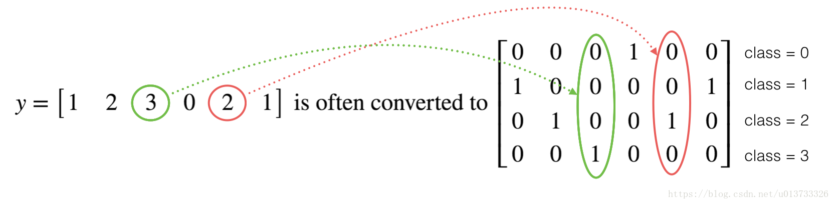
def one_hot_matrix(labels, C):
    """
    Creates a matrix where the i-th row corresponds to the ith class number and the jth column
                     corresponds to the jth training example. So if example j had a label i. Then entry (i,j) 
                     will be 1. 
                     
    Arguments:
    labels -- vector containing the labels 
    C -- number of classes, the depth of the one hot dimension
    
    Returns: 
    one_hot -- one hot matrix
    """
    
    ### START CODE HERE ###
    # Create a tf.constant equal to C (depth), name it 'C'. (approx. 1 line)
    C=tf.constant(C,name='C')
    
    # Use tf.one_hot, be careful with the axis (approx. 1 line)
    one_hot_matrix=tf.one_hot(indices=labels,depth=C,axis=0)
    
    # Create a session (approx. 1 line). See method 1 above.
    sess=tf.Session()
    # Run the session (approx. 1 line).
    one_hot=sess.run(one_hot_matrix)
    # Close the session (approx. 1 line). See method 1 above.
    sess.close()
    ### END CODE HERE ###
    
    return one_hot

1.5初始化

def ones(shape):
    """
    Creates an array of ones of dimension shape
    
    Arguments:
    shape -- shape of the array you want to create
        
    Returns: 
    ones -- array containing only ones
    """
    
    ### START CODE HERE ###   
    # Create "ones" tensor using tf.ones(...). (approx. 1 line)    
    ones=tf.ones(shape)
    
    # Create a session (approx. 1 line). See method 1 above.
    sess=tf.Session()
    # Run the session (approx. 1 line).
    ones=sess.run(ones)
    # Close the session (approx. 1 line). See method 1 above.
    sess.close()
    ### END CODE HERE ###
    
    return ones

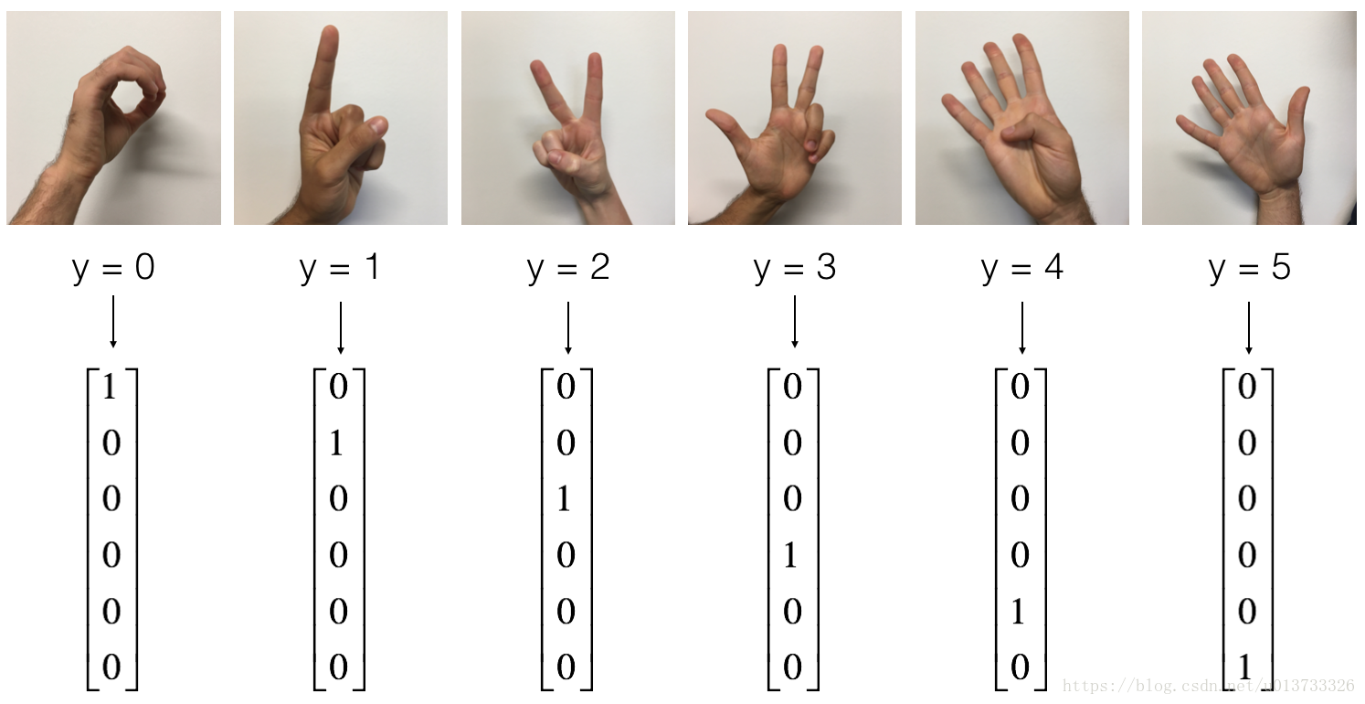
2使用TensorFlow构建神经网络

• 训练集：有从0到5的数字的1080张图片(64x64像素)，每个数字拥有180张图片。
• 测试集：有从0到5的数字的120张图片(64x64像素)，每个数字拥有5张图片。

处理数据

# Loading the dataset
X_train_orig, Y_train_orig, X_test_orig, Y_test_orig, classes = load_dataset()

# Example of a picture
index = 0
plt.imshow(X_train_orig[index])
print ("y = " + str(np.squeeze(Y_train_orig[:, index])))


# Flatten the training and test images
X_train_flatten = X_train_orig.reshape(X_train_orig.shape[0], -1).T
X_test_flatten = X_test_orig.reshape(X_test_orig.shape[0], -1).T
# Normalize image vectors
X_train = X_train_flatten / 255.
X_test = X_test_flatten / 255.
# Convert training and test labels to one hot matrices
Y_train = convert_to_one_hot(Y_train_orig, 6)
Y_test = convert_to_one_hot(Y_test_orig, 6)

print("number of training examples = " + str(X_train.shape[1]))   #1080
print("number of test examples = " + str(X_test.shape[1]))        #120
print("X_train shape: " + str(X_train.shape))             #(12288,1080)
print("Y_train shape: " + str(Y_train.shape))             #(6,1080)
print("X_test shape: " + str(X_test.shape))               #(12288,120)
print("Y_test shape: " + str(Y_test.shape))               #(6,120)

2.1创建placeholders（之后传递数据）

def create_placeholders(n_x, n_y):
    """
    Creates the placeholders for the tensorflow session.
    
    Arguments:
    n_x -- scalar, size of an image vector (num_px * num_px = 64 * 64 * 3 = 12288)
    n_y -- scalar, number of classes (from 0 to 5, so -> 6)
    
    Returns:
    X -- placeholder for the data input, of shape [n_x, None] and dtype "float"
    Y -- placeholder for the input labels, of shape [n_y, None] and dtype "float"
    
    Tips:
    - You will use None because it let's us be flexible on the number of examples you will for the placeholders.
      In fact, the number of examples during test/train is different.
    """

    ### START CODE HERE ### (approx. 2 lines)
    X=tf.placeholder(tf.float32,[n_x,None],name='X')
    Y=tf.placeholder(tf.float32,[n_y,None],name='Y')
    ### END CODE HERE ###
    
    return X, Y

2.2初始化

def initialize_parameters():
    """
    Initializes parameters to build a neural network with tensorflow. The shapes are:
                        W1 : [25, 12288]
                        b1 : [25, 1]
                        W2 : [12, 25]
                        b2 : [12, 1]
                        W3 : [6, 12]
                        b3 : [6, 1]
    
    Returns:
    parameters -- a dictionary of tensors containing W1, b1, W2, b2, W3, b3
    """  
    tf.set_random_seed(1)                   # so that your "random" numbers match ours
        
    ### START CODE HERE ### (approx. 6 lines of code)
    W1 = tf.get_variable("W1",[25,12288],initializer=tf.contrib.layers.xavier_initializer(seed=1))
    b1 = tf.get_variable("b1",[25,1],initializer=tf.zeros_initializer())
    W2 = tf.get_variable("W2", [12, 25], initializer = tf.contrib.layers.xavier_initializer(seed=1))
    b2 = tf.get_variable("b2", [12, 1], initializer = tf.zeros_initializer())
    W3 = tf.get_variable("W3", [6, 12], initializer = tf.contrib.layers.xavier_initializer(seed=1))
    b3 = tf.get_variable("b3", [6, 1], initializer = tf.zeros_initializer())    
    ### END CODE HERE ###

    parameters = {"W1": W1,
                  "b1": b1,
                  "W2": W2,
                  "b2": b2,
                  "W3": W3,
                  "b3": b3}   
    return parameters

2.3Forward propagation

def forward_propagation(X, parameters):
    """
    Implements the forward propagation for the model: LINEAR -> RELU -> LINEAR -> RELU -> LINEAR -> SOFTMAX
    
    Arguments:
    X -- input dataset placeholder, of shape (input size, number of examples)
    parameters -- python dictionary containing your parameters "W1", "b1", "W2", "b2", "W3", "b3"
                  the shapes are given in initialize_parameters

    Returns:
    Z3 -- the output of the last LINEAR unit
    """ 
    # Retrieve the parameters from the dictionary "parameters" 
    W1 = parameters['W1']
    b1 = parameters['b1']
    W2 = parameters['W2']
    b2 = parameters['b2']
    W3 = parameters['W3']
    b3 = parameters['b3']
    
    ### START CODE HERE ### (approx. 5 lines)              # Numpy Equivalents:
    Z1=tf.matmul(W1,X)+b1                       # Z1 = np.dot(W1, X) + b1
    A1=tf.nn.relu(Z1)                           # A1 = relu(Z1)
    Z2=tf.matmul(W2,A1)+b2                      # Z2 = np.dot(W2, a1) + b2
    A2=tf.nn.relu(Z2)                           # A2 = relu(Z2)
    Z3=tf.matmul(W3,A2)+b3                      # Z3 = np.dot(W3,Z2) + b3
    ### END CODE HERE ###
    
    return Z3

2.4计算成本

def compute_cost(Z3, Y):
    """
    Computes the cost
    
    Arguments:
    Z3 -- output of forward propagation (output of the last LINEAR unit), of shape (6, number of examples)
    Y -- "true" labels vector placeholder, same shape as Z3
    
    Returns:
    cost - Tensor of the cost function
    """
    
    # to fit the tensorflow requirement for tf.nn.softmax_cross_entropy_with_logits(...,...)
    logits = tf.transpose(Z3)
    labels = tf.transpose(Y)
    
    ### START CODE HERE ### (1 line of code)
    cost=tf.reduce_mean(tf.nn.softmax_cross_entropy_with_logits(logits=logits, labels=labels))
    ### END CODE HERE ###
    
    return cost

2.5构建模型

def model(X_train, Y_train, X_test, Y_test, learning_rate = 0.0001,
          num_epochs = 1500, minibatch_size = 32, print_cost = True):
    """
    Implements a three-layer tensorflow neural network: LINEAR->RELU->LINEAR->RELU->LINEAR->SOFTMAX.
    
    Arguments:
    X_train -- training set, of shape (input size = 12288, number of training examples = 1080)
    Y_train -- test set, of shape (output size = 6, number of training examples = 1080)
    X_test -- training set, of shape (input size = 12288, number of training examples = 120)
    Y_test -- test set, of shape (output size = 6, number of test examples = 120)
    learning_rate -- learning rate of the optimization
    num_epochs -- number of epochs of the optimization loop
    minibatch_size -- size of a minibatch
    print_cost -- True to print the cost every 100 epochs
    
    Returns:
    parameters -- parameters learnt by the model. They can then be used to predict.
    """
    
    ops.reset_default_graph()                         # to be able to rerun the model without overwriting tf variables
    tf.set_random_seed(1)                             # to keep consistent results
    seed = 3                                          # to keep consistent results
    (n_x, m) = X_train.shape                          # (n_x: input size, m : number of examples in the train set)
    n_y = Y_train.shape[0]                            # n_y : output size
    costs = []                                        # To keep track of the cost
    
    # Create Placeholders of shape (n_x, n_y)
    ### START CODE HERE ### (1 line)
    X,Y=create_placeholders(n_x,n_y)
    ### END CODE HERE ###

    # Initialize parameters
    ### START CODE HERE ### (1 line)
    parameters=initialize_parameters()
    ### END CODE HERE ###
    
    # Forward propagation: Build the forward propagation in the tensorflow graph
    ### START CODE HERE ### (1 line)
    Z3=forward_propagation(X,parameters)
    ### END CODE HERE ###
    
    # Cost function: Add cost function to tensorflow graph
    ### START CODE HERE ### (1 line)
    cost=compute_cost(Z3,Y)
    ### END CODE HERE ###
    
    # Backpropagation: Define the tensorflow optimizer. Use an AdamOptimizer.
    ### START CODE HERE ### (1 line)
    optimizer = tf.train.AdamOptimizer(learning_rate=learning_rate).minimize(cost)
    ### END CODE HERE ###
    
    # Initialize all the variables
    init = tf.global_variables_initializer()

    # Start the session to compute the tensorflow graph
    with tf.Session() as sess:
        
        # Run the initialization
        sess.run(init)
        
        # Do the training loop
        for epoch in range(num_epochs):

            epoch_cost = 0.                       # Defines a cost related to an epoch
            num_minibatches = int(m / minibatch_size) # number of minibatches of size minibatch_size in the train set
            seed = seed + 1
            minibatches = random_mini_batches(X_train, Y_train, minibatch_size, seed)

            for minibatch in minibatches:

                # Select a minibatch
                (minibatch_X, minibatch_Y) = minibatch
                
                # IMPORTANT: The line that runs the graph on a minibatch.
                # Run the session to execute the "optimizer" and the "cost", the feedict should contain a minibatch for (X,Y).
                ### START CODE HERE ### (1 line)
                _ , minibatch_cost = sess.run([optimizer, cost], feed_dict={X: minibatch_X, Y: minibatch_Y})
                ### END CODE HERE ###
                
                epoch_cost += minibatch_cost / num_minibatches

            # Print the cost every epoch
            if print_cost == True and epoch % 100 == 0:
                print ("Cost after epoch %i: %f" % (epoch, epoch_cost))
            if print_cost == True and epoch % 5 == 0:
                costs.append(epoch_cost)
                
        # plot the cost
        plt.plot(np.squeeze(costs))
        plt.ylabel('cost')
        plt.xlabel('iterations (per tens)')
        plt.title("Learning rate =" + str(learning_rate))
        plt.show()

        # lets save the parameters in a variable
        parameters = sess.run(parameters)
        print("Parameters have been trained!")

        # Calculate the correct predictions
        correct_prediction = tf.equal(tf.argmax(Z3), tf.argmax(Y))

        # Calculate accuracy on the test set
        accuracy = tf.reduce_mean(tf.cast(correct_prediction, "float"))

        print("Train Accuracy:", accuracy.eval({X: X_train, Y: Y_train}))
        print("Test Accuracy:", accuracy.eval({X: X_test, Y: Y_test}))
        
        return parameters  

 

Parameters have been trained!
Train Accuracy: 0.999074
Test Accuracy: 0.725