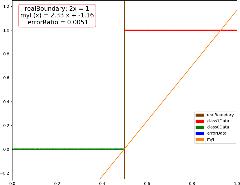
▶ 感知机来找到线性可分数据集的分割,很像单层神经网络
● 原始形式感知机,代码
  1 import numpy as np
  2 import matplotlib.pyplot as plt
  3 from mpl_toolkits.mplot3d import Axes3D
  4 from mpl_toolkits.mplot3d.art3d import Poly3DCollection
  5 from matplotlib.patches import Rectangle
  6 import warnings
  7
  8 warnings.filterwarnings("ignore")
  9 dataSize = 10000
 10 trainRatio = 0.3
 11 maxTurn = 300
 12 ita = 0.3
 13 epsilon = 0.01
 14 colors = [[0.5,0.25,0],[1,0,0],[0,0.5,0],[0,0,1],[1,0.5,0]]                         # 棕红绿蓝橙
 15 trans = 0.5
 16
 17 def dataSplit(x, y, part):                                                          # 将数据集按给定索引分为两段
 18     return x[:part], y[:part],x[part:],y[part:]
 19
 20 def function(x,para):                                                               # 回归函数
 21     return np.sum(x * para[0]) + para[1]
 22
 23 def judge(x, para):                                                                 # 分类函数,由乘加部分和阈值部分组成
 24     return np.sign(function(x, para))
 25
 26 def createData(dim, count = dataSize):                                              # 创建数据集
 27     np.random.seed(103)
 28     X = np.random.rand(count,dim)
 29     Y = 2 * ((3 - 2 * dim)*X[:,0] + 2 * np.sum(X[:,1:], 1) > 0.5).astype(int) - 1   # 只考虑 {-1,1} 的二分类
 30     #print(output)
 31     class1Count = 0
 32     for i in range(count):
 33         class1Count += (Y[i] + 1)>>1
 34     print("dim = %d, dataSize = %d, class 1 count -> %4f"%(dim, count, class1Count / count))
 35     return X, Y
 36
 37 def perceptron(dataX, dataY):                                                       # 感知机
 38     count, dim = np.shape(dataX)
 39     w = np.random.rand(dim)                                                         # 随机初值
 40     b = np.random.rand()
 41
 42     turn = 0
 43     while turn < maxTurn:
 44         error = 0.0
 45         for i in range(count):
 46             if dataY[i] * (np.sum(w * dataX[i]) + b) <= 0:                          # 找到分类错误的点
 47                 w += ita * dataX[i] * dataY[i]                                      # 修正 w 和 b
 48                 b += ita *dataY[i]
 49                 error += np.sum(w * dataX[i] + b - dataY[i]) ** 2
 50         error /= count
 51         turn += 1
 52         print("turn = ", turn, ", error = ", error)
 53         if error < epsilon:
 54             break
 55     return (w, b)
 56
 57 def test(dim):
 58     allX, allY = createData(dim)
 59     trainX, trainY, testX, testY = dataSplit(allX, allY, int(dataSize * trainRatio))
 60
 61     para = perceptron(trainX, trainY)
 62
 63     myResult = [ judge(x, para) for x in testX]                                     # 测试结果
 64     errorRatio = np.sum((np.array(myResult) - testY)**2) / (dataSize * (1 - trainRatio))
 65     print("dim = %d, errorRatio = %4f
"%(dim, errorRatio))
 66
 67     if dim >= 4:                                                                    # 4维以上不画图,只输出测试错误率
 68         return
 69     errorPX = []                                                                    # 测试数据集分为错误类,1 类和 0 类
 70     errorPY = []
 71     class1 = []
 72     class0 = []
 73     for i in range(len(testX)):
 74         if myResult[i] != testY[i]:
 75             errorPX.append(testX[i])
 76             errorPY.append(testY[i])
 77         elif myResult[i] == 1:
 78             class1.append(testX[i])
 79         else:
 80             class0.append(testX[i])
 81     errorPX = np.array(errorPX)
 82     errorPY = np.array(errorPY)
 83     class1 = np.array(class1)
 84     class0 = np.array(class0)
 85
 86     fig = plt.figure(figsize=(10, 8))
 87
 88     if dim == 1:
 89         plt.xlim(0.0,1.0)
 90         plt.ylim(-0.25,1.25)
 91         plt.plot([0.5, 0.5], [-0.5, 1.25], color = colors[0],label = "realBoundary")
 92         plt.plot([0, 1], [ function(i, para) for i in [0,1] ],color = colors[4], label = "myF")
 93         plt.scatter(class1, np.ones(len(class1)), color = colors[1], s = 2,label = "class1Data")
 94         plt.scatter(class0, np.zeros(len(class0)), color = colors[2], s = 2,label = "class0Data")
 95         if len(errorPX) != 0:
 96             plt.scatter(errorPX, errorPY,color = colors[3], s = 16,label = "errorData")
 97         plt.text(0.2, 1.12, "realBoundary: 2x = 1
myF(x) = " + str(round(para[0][0],2)) + " x + " + str(round(para[1],2)) + "
 errorRatio = " + str(round(errorRatio,4)),
 98             size=15, ha="center", va="center", bbox=dict(boxstyle="round", ec=(1., 0.5, 0.5), fc=(1., 1., 1.)))
 99         R = [Rectangle((0,0),0,0, color = colors[k]) for k in range(5)]
100         plt.legend(R, ["realBoundary", "class1Data", "class0Data", "errorData", "myF"], loc=[0.81, 0.2], ncol=1, numpoints=1, framealpha = 1)
101
102     if dim == 2:
103         plt.xlim(0.0,1.0)
104         plt.ylim(0.0,1.0)
105         plt.plot([0,1], [0.25,0.75], color = colors[0],label = "realBoundary")
106         xx = np.arange(0, 1 + 0.1, 0.1)
107         X,Y = np.meshgrid(xx, xx)
108         contour = plt.contour(X, Y, [ [ function((X[i,j],Y[i,j]), para) for j in range(11)] for i in range(11) ])
109         plt.clabel(contour, fontsize = 10,colors='k')
110         plt.scatter(class1[:,0], class1[:,1], color = colors[1], s = 2,label = "class1Data")
111         plt.scatter(class0[:,0], class0[:,1], color = colors[2], s = 2,label = "class0Data")
112         if len(errorPX) != 0:
113             plt.scatter(errorPX[:,0], errorPX[:,1], color = colors[3], s = 8,label = "errorData")
114         plt.text(0.73, 0.92, "realBoundary: -x + 2y = 1/2
myF(x,y) = " + str(round(para[0][0],2)) + " x + " + str(round(para[0][1],2)) + " y + " + str(round(para[1],2)) + "
 errorRatio = " + str(round(errorRatio,4)),
115             size = 15, ha="center", va="center", bbox=dict(boxstyle="round", ec=(1., 0.5, 0.5), fc=(1., 1., 1.)))
116         R = [Rectangle((0,0),0,0, color = colors[k]) for k in range(4)]
117         plt.legend(R, ["realBoundary", "class1Data", "class0Data", "errorData"], loc=[0.81, 0.2], ncol=1, numpoints=1, framealpha = 1)
118
119     if dim == 3:
120         ax = Axes3D(fig)
121         ax.set_xlim3d(0.0, 1.0)
122         ax.set_ylim3d(0.0, 1.0)
123         ax.set_zlim3d(0.0, 1.0)
124         ax.set_xlabel('X', fontdict={'size': 15, 'color': 'k'})
125         ax.set_ylabel('Y', fontdict={'size': 15, 'color': 'k'})
126         ax.set_zlabel('W', fontdict={'size': 15, 'color': 'k'})
127         v = [(0, 0, 0.25), (0, 0.25, 0), (0.5, 1, 0), (1, 1, 0.75), (1, 0.75, 1), (0.5, 0, 1)]
128         f = [[0,1,2,3,4,5]]
129         poly3d = [[v[i] for i in j] for j in f]
130         ax.add_collection3d(Poly3DCollection(poly3d, edgecolor = 'k', facecolors = colors[0]+[trans], linewidths=1))
131         ax.scatter(class1[:,0], class1[:,1],class1[:,2], color = colors[1], s = 2, label = "class1")
132         ax.scatter(class0[:,0], class0[:,1],class0[:,2], color = colors[2], s = 2, label = "class0")
133         if len(errorPX) != 0:
134             ax.scatter(errorPX[:,0], errorPX[:,1],errorPX[:,2], color = colors[3], s = 8, label = "errorData")
135         ax.text3D(0.8, 0.98, 1.15, "realBoundary: -3x + 2y +2z = 1/2
myF(x,y,z) = " + str(round(para[0][0],2)) + " x + " +
136             str(round(para[0][1],2)) + " y + " + str(round(para[0][2],2)) + " z + " + str(round(para[1],2)) + "
 errorRatio = " + str(round(errorRatio,4)),
137             size = 12, ha="center", va="center", bbox=dict(boxstyle="round", ec=(1, 0.5, 0.5), fc=(1, 1, 1)))
138         R = [Rectangle((0,0),0,0, color = colors[k]) for k in range(4)]
139         plt.legend(R, ["realBoundary", "class1Data", "class0Data", "errorData"], loc=[0.83, 0.1], ncol=1, numpoints=1, framealpha = 1)
140
141     fig.savefig("R:\dim" + str(dim) + ".png")
142     plt.close()
143
144 if __name__ == '__main__':
145     test(1)
146     test(2)
147     test(3)
148     test(4)
● 输出结果
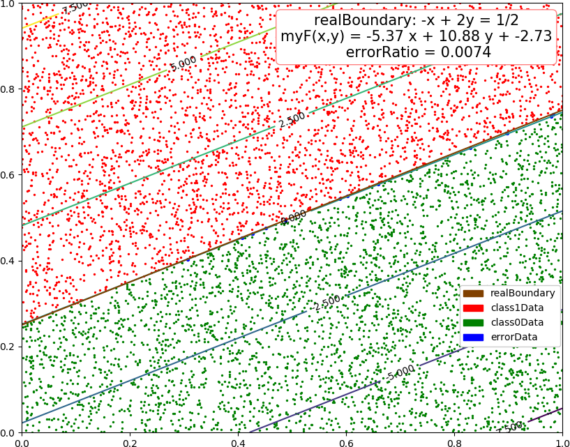
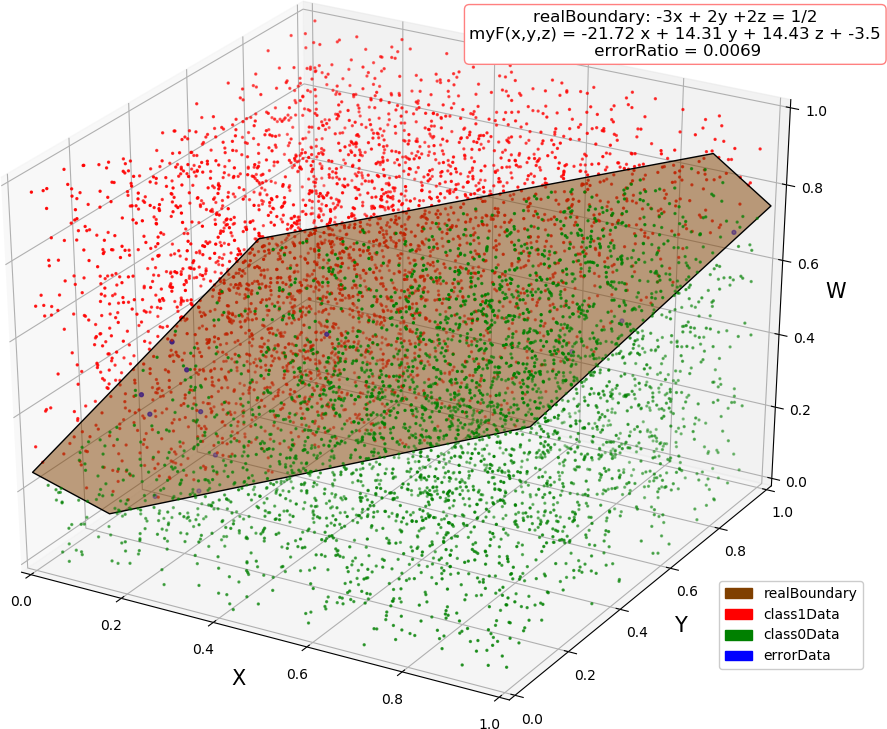
dim = 1, dataSize = 10000, class 1 count -> 0.509000
turn =  1 , error =  0.017389410798594473
turn =  2 , error =  0.0
dim = 1, errorRatio = 0.004571

dim = 2, dataSize = 10000, class 1 count -> 0.496000
turn =  1 , error =  0.21416356258715985

...

turn =  11 , error =  0.10398373598573663
turn =  12 , error =  0.045706020341763055
turn =  13 , error =  0.0
dim = 2, errorRatio = 0.002286

dim = 3, dataSize = 10000, class 1 count -> 0.498200
turn =  1 , error =  0.45650719829126757

...

turn =  12 , error =  0.14528529033345788
turn =  13 , error =  0.1376817605623497
turn =  14 , error =  0.0
dim = 3, errorRatio = 0.000571

dim = 4, dataSize = 10000, class 1 count -> 0.496900
turn =  1 , error =  0.7717105869223287

...

turn =  298 , error =  0.7316455346511096
turn =  299 , error =  0.6088039354340593
turn =  300 , error =  0.48205216369651693
dim = 4, errorRatio = 0.005143
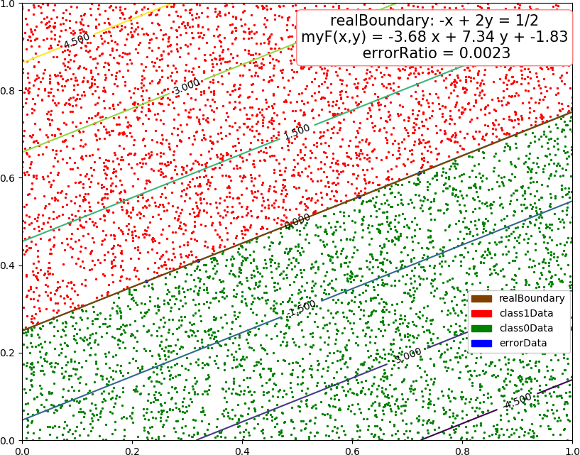
● 画图
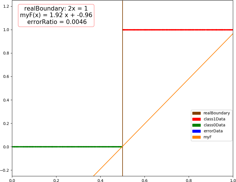

● 对偶形式感知机,代码,只改变函数 perceptron,不用 Gram 矩阵,太占空间
 1 def perceptron(dataX, dataY):
 2     count, dim = np.shape(dataX)
 3     w = np.random.rand(dim)                                                         # 随机初值
 4     b = np.random.rand()
 5     alpha = np.zeros(count)
 6     xy = dataX * dataY.reshape(count,1)
 7
 8     turn = 0
 9     while turn < maxTurn:
10         error = 0.0
11         for i in range(count):
12             t = np.sum(np.matmul(alpha,xy) * dataX[i]) + b                           # 当前预测值
13             if dataY[i] * t <= 0:                                                    # 选取分类错误的点进行修正
14                 alpha[i] += ita
15                 b += ita * dataY[i]
16
17         w = np.matmul(alpha,xy)                                                      # 一轮结束,计算 w 和误差
18         error = np.sum( (np.sign(np.sum(w * dataX, 1) + b) - dataY) ** 2 ) / count
19         turn += 1
20         print("turn = ", turn, ", error = ", error)
21         if error < epsilon:
22             break
23     return (w, b)
● 输出结果,似乎更快,但是精度有所下降
dim = 1, dataSize = 10000, class 1 count -> 0.509000
turn =  1 , error =  0.0
dim = 1, errorRatio = 0.005143

dim = 2, dataSize = 10000, class 1 count -> 0.496000
turn =  1 , error =  0.008
dim = 2, errorRatio = 0.007429

dim = 3, dataSize = 10000, class 1 count -> 0.498200
turn =  1 , error =  0.07333333333333333
turn =  2 , error =  0.3293333333333333
turn =  3 , error =  0.018666666666666668
turn =  4 , error =  0.012
turn =  5 , error =  0.172
turn =  6 , error =  0.10666666666666667
turn =  7 , error =  0.05333333333333334
turn =  8 , error =  0.0026666666666666666
dim = 3, errorRatio = 0.006857

dim = 4, dataSize = 10000, class 1 count -> 0.496900
turn =  1 , error =  0.088

...

turn =  45 , error =  0.021333333333333333
turn =  46 , error =  0.009333333333333334
dim = 4, errorRatio = 0.010857
● 画图