题目要求
根据学生两门课的成绩和是否入学的数据,预测学生能否顺利入学:利用ex2data1.txt和ex2data2.txt中的数据,进行逻辑回归和预测。
数据放在最后边。
ex2data1.txt处理
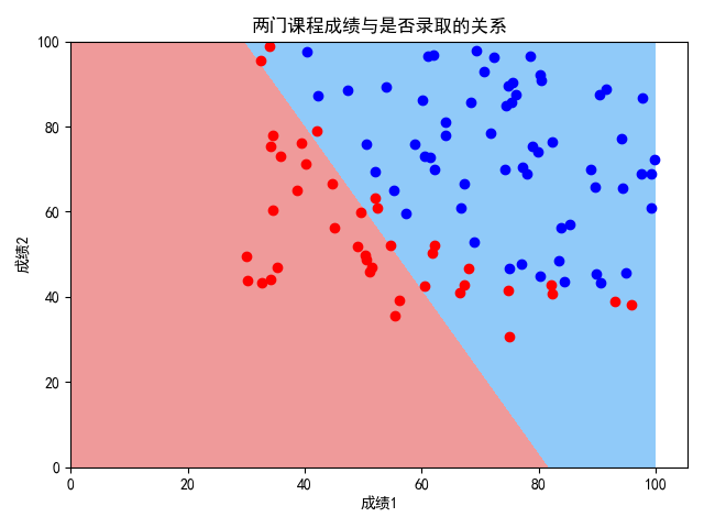
作散点图可知,决策大致符合线性关系,但还是有弯曲(非线性),用线性效果并不好,因此可用两种方案:方案一,无多项式特征;方案二,有多项式特征。
方案一:无多项式特征
对ex2data1.txt中的数据进行逻辑回归,无多项式特征
代码实现如下:
"""
    对ex2data1.txt中的数据进行逻辑回归(无多项式特征)
"""
from sklearn.model_selection import train_test_split
from matplotlib.colors import ListedColormap
from sklearn.linear_model import LogisticRegression
import numpy as np
import matplotlib.pyplot as plt
plt.rcParams['font.sans-serif'] = ['SimHei']  # 用来正常显示中文标签
plt.rcParams['axes.unicode_minus'] = False  # 用来正常显示负号

# 数据格式:成绩1,成绩2,是否被录取(1代表被录取,0代表未被录取)


# 函数(画决策边界)定义
def plot_decision_boundary(model, axis):
    x0, x1 = np.meshgrid(
        np.linspace(axis[0], axis[1], int((axis[1] - axis[0]) * 100)).reshape(-1, 1),
        np.linspace(axis[2], axis[3], int((axis[3] - axis[2]) * 100)).reshape(-1, 1),
    )
    X_new = np.c_[x0.ravel(), x1.ravel()]

    y_predict = model.predict(X_new)
    zz = y_predict.reshape(x0.shape)

    custom_cmap = ListedColormap(['#EF9A9A', '#FFF59D', '#90CAF9'])

    plt.contourf(x0, x1, zz, cmap=custom_cmap)

# 读取数据
data = np.loadtxt('ex2data1.txt', delimiter=',')
data_X = data[:, 0:2]
data_y = data[:, 2]

# 数据分割
X_train, X_test, y_train, y_test = train_test_split(data_X, data_y, random_state=666)

# 训练模型
log_reg = LogisticRegression()
log_reg.fit(X_train, y_train)

# 结果可视化
plot_decision_boundary(log_reg, axis=[0, 100, 0, 100])
plt.scatter(data_X[data_y == 0, 0], data_X[data_y == 0, 1], color='red')
plt.scatter(data_X[data_y == 1, 0], data_X[data_y == 1, 1], color='blue')
plt.xlabel('成绩1')
plt.ylabel('成绩2')
plt.title('两门课程成绩与是否录取的关系')
plt.show()

# 模型测试
print(log_reg.score(X_train, y_train))
print(log_reg.score(X_test, y_test))
输出结果如下:
0.8533333333333334
0.76
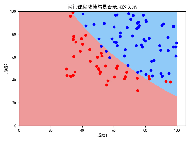
方案二:引入多项式特征
对ex2data1.txt中的数据进行逻辑回归,引入多项式特征。经调试,当degree为3时,耗费时间较长;当degree为2时,耗费时间可接受,效果与方案一相比好了很多
实现如下:
"""
    对ex2data1.txt中的数据进行逻辑回归(引入多项式特征)
"""
from sklearn.model_selection import train_test_split
from matplotlib.colors import ListedColormap
from sklearn.linear_model import LogisticRegression
import numpy as np
import matplotlib.pyplot as plt
from sklearn.preprocessing import PolynomialFeatures
from sklearn.pipeline import Pipeline
from sklearn.preprocessing import StandardScaler
plt.rcParams['font.sans-serif'] = ['SimHei']  # 用来正常显示中文标签
plt.rcParams['axes.unicode_minus'] = False  # 用来正常显示负号

# 数据格式:成绩1,成绩2,是否被录取(1代表被录取,0代表未被录取)


# 函数定义
def plot_decision_boundary(model, axis):
    x0, x1 = np.meshgrid(
        np.linspace(axis[0], axis[1], int((axis[1] - axis[0]) * 100)).reshape(-1, 1),
        np.linspace(axis[2], axis[3], int((axis[3] - axis[2]) * 100)).reshape(-1, 1),
    )
    X_new = np.c_[x0.ravel(), x1.ravel()]

    y_predict = model.predict(X_new)
    zz = y_predict.reshape(x0.shape)

    custom_cmap = ListedColormap(['#EF9A9A', '#FFF59D', '#90CAF9'])

    plt.contourf(x0, x1, zz, cmap=custom_cmap)


def PolynomialLogisticRegression(degree):
    return Pipeline([
        ('poly', PolynomialFeatures(degree=degree)),
        ('std_scaler', StandardScaler()),
        ('log_reg', LogisticRegression())
    ])


# 读取数据
data = np.loadtxt('ex2data1.txt', delimiter=',')
data_X = data[:, 0:2]
data_y = data[:, 2]

# 数据分割
X_train, X_test, y_train, y_test = train_test_split(data_X, data_y, random_state=666)

# 训练模型
poly_log_reg = PolynomialLogisticRegression(degree=2)
poly_log_reg.fit(X_train, y_train)

# 结果可视化
plot_decision_boundary(poly_log_reg, axis=[0, 100, 0, 100])
plt.scatter(data_X[data_y == 0, 0], data_X[data_y == 0, 1], color='red')
plt.scatter(data_X[data_y == 1, 0], data_X[data_y == 1, 1], color='blue')
plt.xlabel('成绩1')
plt.ylabel('成绩2')
plt.title('两门课程成绩与是否录取的关系')
plt.show()

# 模型测试
print(poly_log_reg.score(X_train, y_train))
print(poly_log_reg.score(X_test, y_test))
输出如下:
0.92
0.92
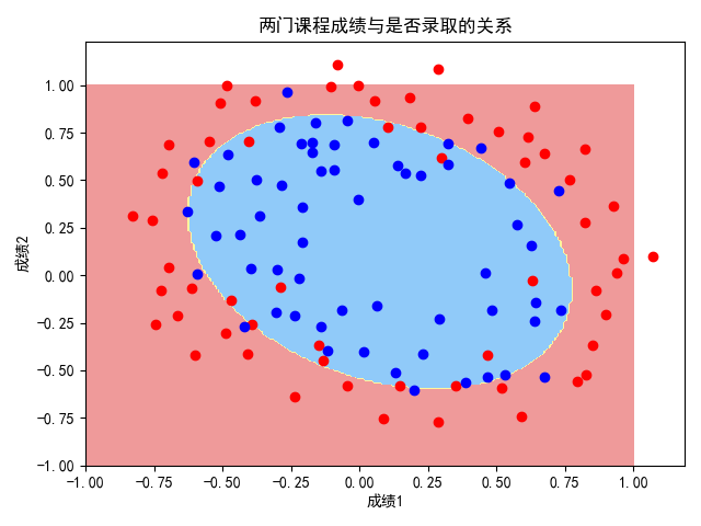
ex2data2.txt处理
作散点图可知,这组数据的决策边界绝对是非线性的,所以直接引入多项式特征对ex2data2.txt中的数据进行逻辑回归。
代码实现如下:
"""
    对ex2data2.txt中的数据进行逻辑回归(引入多项式特征)
"""
from sklearn.model_selection import train_test_split
from matplotlib.colors import ListedColormap
from sklearn.linear_model import LogisticRegression
import numpy as np
import matplotlib.pyplot as plt
from sklearn.preprocessing import PolynomialFeatures
from sklearn.pipeline import Pipeline
from sklearn.preprocessing import StandardScaler
plt.rcParams['font.sans-serif'] = ['SimHei']  # 用来正常显示中文标签
plt.rcParams['axes.unicode_minus'] = False  # 用来正常显示负号

# 数据格式:成绩1,成绩2,是否被录取(1代表被录取,0代表未被录取)


# 函数定义
def plot_decision_boundary(model, axis):
    x0, x1 = np.meshgrid(
        np.linspace(axis[0], axis[1], int((axis[1] - axis[0]) * 100)).reshape(-1, 1),
        np.linspace(axis[2], axis[3], int((axis[3] - axis[2]) * 100)).reshape(-1, 1),
    )
    X_new = np.c_[x0.ravel(), x1.ravel()]

    y_predict = model.predict(X_new)
    zz = y_predict.reshape(x0.shape)

    custom_cmap = ListedColormap(['#EF9A9A', '#FFF59D', '#90CAF9'])

    plt.contourf(x0, x1, zz, cmap=custom_cmap)


def PolynomialLogisticRegression(degree):
    return Pipeline([
        ('poly', PolynomialFeatures(degree=degree)),
        ('std_scaler', StandardScaler()),
        ('log_reg', LogisticRegression())
    ])


# 读取数据
data = np.loadtxt('ex2data2.txt', delimiter=',')
data_X = data[:, 0:2]
data_y = data[:, 2]

# 数据分割
X_train, X_test, y_train, y_test = train_test_split(data_X, data_y, random_state=666)

# 训练模型
poly_log_reg = PolynomialLogisticRegression(degree=2)
poly_log_reg.fit(X_train, y_train)

# 结果可视化
plot_decision_boundary(poly_log_reg, axis=[-1, 1, -1, 1])
plt.scatter(data_X[data_y == 0, 0], data_X[data_y == 0, 1], color='red')
plt.scatter(data_X[data_y == 1, 0], data_X[data_y == 1, 1], color='blue')
plt.xlabel('成绩1')
plt.ylabel('成绩2')
plt.title('两门课程成绩与是否录取的关系')
plt.show()

# 模型测试
print(poly_log_reg.score(X_train, y_train))
print(poly_log_reg.score(X_test, y_test))
输出结果如下:
由图可知,分类结果较好。
0.7954545454545454
0.9
两份数据
ex2data1.txt
34.62365962451697,78.0246928153624,0
30.28671076822607,43.89499752400101,0
35.84740876993872,72.90219802708364,0
60.18259938620976,86.30855209546826,1
79.0327360507101,75.3443764369103,1
45.08327747668339,56.3163717815305,0
61.10666453684766,96.51142588489624,1
75.02474556738889,46.55401354116538,1
76.09878670226257,87.42056971926803,1
84.43281996120035,43.53339331072109,1
95.86155507093572,38.22527805795094,0
75.01365838958247,30.60326323428011,0
82.30705337399482,76.48196330235604,1
69.36458875970939,97.71869196188608,1
39.53833914367223,76.03681085115882,0
53.9710521485623,89.20735013750205,1
69.07014406283025,52.74046973016765,1
67.94685547711617,46.67857410673128,0
70.66150955499435,92.92713789364831,1
76.97878372747498,47.57596364975532,1
67.37202754570876,42.83843832029179,0
89.67677575072079,65.79936592745237,1
50.534788289883,48.85581152764205,0
34.21206097786789,44.20952859866288,0
77.9240914545704,68.9723599933059,1
62.27101367004632,69.95445795447587,1
80.1901807509566,44.82162893218353,1
93.114388797442,38.80067033713209,0
61.83020602312595,50.25610789244621,0
38.78580379679423,64.99568095539578,0
61.379289447425,72.80788731317097,1
85.40451939411645,57.05198397627122,1
52.10797973193984,63.12762376881715,0
52.04540476831827,69.43286012045222,1
40.23689373545111,71.16774802184875,0
54.63510555424817,52.21388588061123,0
33.91550010906887,98.86943574220611,0
64.17698887494485,80.90806058670817,1
74.78925295941542,41.57341522824434,0
34.1836400264419,75.2377203360134,0
83.90239366249155,56.30804621605327,1
51.54772026906181,46.85629026349976,0
94.44336776917852,65.56892160559052,1
82.36875375713919,40.61825515970618,0
51.04775177128865,45.82270145776001,0
62.22267576120188,52.06099194836679,0
77.19303492601364,70.45820000180959,1
97.77159928000232,86.7278223300282,1
62.07306379667647,96.76882412413983,1
91.56497449807442,88.69629254546599,1
79.94481794066932,74.16311935043758,1
99.2725269292572,60.99903099844988,1
90.54671411399852,43.39060180650027,1
34.52451385320009,60.39634245837173,0
50.2864961189907,49.80453881323059,0
49.58667721632031,59.80895099453265,0
97.64563396007767,68.86157272420604,1
32.57720016809309,95.59854761387875,0
74.24869136721598,69.82457122657193,1
71.79646205863379,78.45356224515052,1
75.3956114656803,85.75993667331619,1
35.28611281526193,47.02051394723416,0
56.25381749711624,39.26147251058019,0
30.05882244669796,49.59297386723685,0
44.66826172480893,66.45008614558913,0
66.56089447242954,41.09209807936973,0
40.45755098375164,97.53518548909936,1
49.07256321908844,51.88321182073966,0
80.27957401466998,92.11606081344084,1
66.74671856944039,60.99139402740988,1
32.72283304060323,43.30717306430063,0
64.0393204150601,78.03168802018232,1
72.34649422579923,96.22759296761404,1
60.45788573918959,73.09499809758037,1
58.84095621726802,75.85844831279042,1
99.82785779692128,72.36925193383885,1
47.26426910848174,88.47586499559782,1
50.45815980285988,75.80985952982456,1
60.45555629271532,42.50840943572217,0
82.22666157785568,42.71987853716458,0
88.9138964166533,69.80378889835472,1
94.83450672430196,45.69430680250754,1
67.31925746917527,66.58935317747915,1
57.23870631569862,59.51428198012956,1
80.36675600171273,90.96014789746954,1
68.46852178591112,85.59430710452014,1
42.0754545384731,78.84478600148043,0
75.47770200533905,90.42453899753964,1
78.63542434898018,96.64742716885644,1
52.34800398794107,60.76950525602592,0
94.09433112516793,77.15910509073893,1
90.44855097096364,87.50879176484702,1
55.48216114069585,35.57070347228866,0
74.49269241843041,84.84513684930135,1
89.84580670720979,45.35828361091658,1
83.48916274498238,48.38028579728175,1
42.2617008099817,87.10385094025457,1
99.31500880510394,68.77540947206617,1
55.34001756003703,64.9319380069486,1
74.77589300092767,89.52981289513276,1
ex2data2.txt
0.051267,0.69956,1
-0.092742,0.68494,1
-0.21371,0.69225,1
-0.375,0.50219,1
-0.51325,0.46564,1
-0.52477,0.2098,1
-0.39804,0.034357,1
-0.30588,-0.19225,1
0.016705,-0.40424,1
0.13191,-0.51389,1
0.38537,-0.56506,1
0.52938,-0.5212,1
0.63882,-0.24342,1
0.73675,-0.18494,1
0.54666,0.48757,1
0.322,0.5826,1
0.16647,0.53874,1
-0.046659,0.81652,1
-0.17339,0.69956,1
-0.47869,0.63377,1
-0.60541,0.59722,1
-0.62846,0.33406,1
-0.59389,0.005117,1
-0.42108,-0.27266,1
-0.11578,-0.39693,1
0.20104,-0.60161,1
0.46601,-0.53582,1
0.67339,-0.53582,1
-0.13882,0.54605,1
-0.29435,0.77997,1
-0.26555,0.96272,1
-0.16187,0.8019,1
-0.17339,0.64839,1
-0.28283,0.47295,1
-0.36348,0.31213,1
-0.30012,0.027047,1
-0.23675,-0.21418,1
-0.06394,-0.18494,1
0.062788,-0.16301,1
0.22984,-0.41155,1
0.2932,-0.2288,1
0.48329,-0.18494,1
0.64459,-0.14108,1
0.46025,0.012427,1
0.6273,0.15863,1
0.57546,0.26827,1
0.72523,0.44371,1
0.22408,0.52412,1
0.44297,0.67032,1
0.322,0.69225,1
0.13767,0.57529,1
-0.0063364,0.39985,1
-0.092742,0.55336,1
-0.20795,0.35599,1
-0.20795,0.17325,1
-0.43836,0.21711,1
-0.21947,-0.016813,1
-0.13882,-0.27266,1
0.18376,0.93348,0
0.22408,0.77997,0
0.29896,0.61915,0
0.50634,0.75804,0
0.61578,0.7288,0
0.60426,0.59722,0
0.76555,0.50219,0
0.92684,0.3633,0
0.82316,0.27558,0
0.96141,0.085526,0
0.93836,0.012427,0
0.86348,-0.082602,0
0.89804,-0.20687,0
0.85196,-0.36769,0
0.82892,-0.5212,0
0.79435,-0.55775,0
0.59274,-0.7405,0
0.51786,-0.5943,0
0.46601,-0.41886,0
0.35081,-0.57968,0
0.28744,-0.76974,0
0.085829,-0.75512,0
0.14919,-0.57968,0
-0.13306,-0.4481,0
-0.40956,-0.41155,0
-0.39228,-0.25804,0
-0.74366,-0.25804,0
-0.69758,0.041667,0
-0.75518,0.2902,0
-0.69758,0.68494,0
-0.4038,0.70687,0
-0.38076,0.91886,0
-0.50749,0.90424,0
-0.54781,0.70687,0
0.10311,0.77997,0
0.057028,0.91886,0
-0.10426,0.99196,0
-0.081221,1.1089,0
0.28744,1.087,0
0.39689,0.82383,0
0.63882,0.88962,0
0.82316,0.66301,0
0.67339,0.64108,0
1.0709,0.10015,0
-0.046659,-0.57968,0
-0.23675,-0.63816,0
-0.15035,-0.36769,0
-0.49021,-0.3019,0
-0.46717,-0.13377,0
-0.28859,-0.060673,0
-0.61118,-0.067982,0
-0.66302,-0.21418,0
-0.59965,-0.41886,0
-0.72638,-0.082602,0
-0.83007,0.31213,0
-0.72062,0.53874,0
-0.59389,0.49488,0
-0.48445,0.99927,0
-0.0063364,0.99927,0
0.63265,-0.030612,0
作者:@臭咸鱼
转载请注明出处:https://www.cnblogs.com/chouxianyu/
欢迎讨论和交流!