CNN模型合集 | 1 LeNet

1.1 LeNet的设计思想
1998年LeCun提出，经典结构，3层，五脏俱全（卷积层、Pooling层、FC网络、Sigmod层），对标传统神经网络。
主要设计贡献

• 局部感受野(local receptive fields)，局部连接
• 权值共享（参数共享）
• 下采样(sub-sampling)，pooling层

核心结构

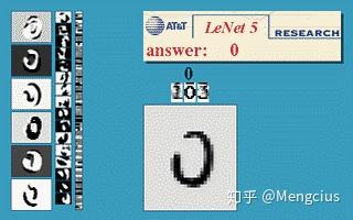
LeNet-5是LeCun最新的卷积网络，专为手写和机器打印的字符识别而设计，下面是LeNet-5实际应用的一个例子。

传统网络的全连接FC（VS局部连接）

• 传统神经网络连接方式是通过全连接，上一层的所有神经元节点x会和下一层的每一个节点y进行互连，线性变换y=w*x_all+b
• 权值参数多，系统开销大，稠密
• 对平移、形变不具有不变性，对局部信息不敏感，完全忽略了图像的局部结构，因为考虑到了所有点。
• 图如果发生一点变化就会导致输出结果产生很大差异（病态问题：对输入输出敏不敏感，收集到是数据往往带有噪声，若模型对此偏差敏感就是病态系统，不鲁棒）
• 全连接相当于1*1的卷积核

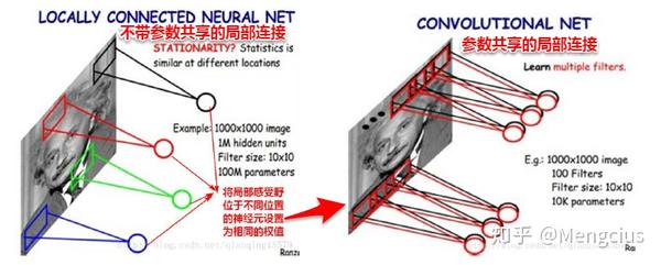
参数共享的局部连接（VS纯局部连接还是不够好，想进一步减少参数规模）

• 减小参数规模，如下图参数共享的局部连接参数减少到了10k，后阶段做模型时越小越好，大的话终端运行时空间很大加载会很慢，很占内存。
• 参数共享就是每种(个)filter学习一种feature，同一种filter权值当然是共享，所有的局部感受野就是用同一种参数，所以就每个卷积层需要很多种filter，也就是depth来学习很多种不同的特征。
• 用一组固定的参数和不同窗口做卷积，来得到下一层特征。每一种滤波器（卷积）就是一种特征，就像高斯滤波等保留了高频或低频的信号。
• 神经网络的卷积就是用一种滤波器提取一种特征，学习多种滤波器，保证多样性；又在经过下采样的不同层上来学习不同滤波器，这样就在不同的力度上提取了不同的特征，比较完善。

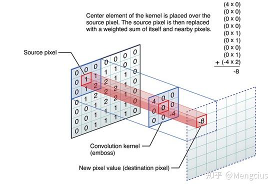
卷积

• 感受野下的各像素与卷积核相乘，再相加赋给中心像素。
• 傅里叶变换与信号处理的知识，跟高斯滤波、锐化、边缘检测等一样提取高频信号。
• 边缘检测时手动设计卷积核为按

  欢迎光临程序代写小店https://item.taobao.com/item.htm?spm=a230r.1.14.59.255028c3ALNkZ0&id=586797758241&ns=1&abbucket=15#detail
  可直接联系客服QQ交代需求：953586085

  列递减的值[[1,0,-1], [1,0,-1],[1,0,-1]]，与它相乘就相当于左边的像素减去右边的，就能检测出垂直边缘信息。以前传统机器学习是手动设计卷积核特征（如颜色信息、纹理信息、形状信息）。

下采样(sub-sampling)，pooling层

• 缩小图像，但不会长宽比形变（区别resize），获得多尺度的信息，以免单一，相当于均值滤波器
• 忽略目标的倾斜、旋转之类的相对位置的变化，以此提高精度，不管怎么转获得的最大值会均值都是不变的
• 降低了特征图的维度，推理时能适应多尺度的图像，
• 可以避免过拟合，因为维度小了，参数少了，计算量少了

Sigmod层

• 连续的函数，这里分类用，逼近不可导的0-1阶跃激活函数，高斯连接，逻辑回归函数，1维的，输出是0~1间的数
• 而常用的Softmax是2维的，输出是2个概率值，正样本的概率和负样本的概率。程序代写接单群733065427
  
  1.2 Caffe实现LeNet
  参考：https://github.com/XuekuanWang/demoCaffe 或者 https://github.com/BVLC/caffe/tree/master/examples/mnist 或者 https://github.com/jklhj222/caffe_LeNet/tree/master/LeNet
  （1）lenet_solver.prototxt 训练参数
• net：网络模型文件的路径
• test_iter：在测试的时候需要迭代的次数，即test_iter* batchsize（测试集的）=测试集的大小，测试集batchsize可以在tran_test.prototxt文件里设置
• test_interval：测试间隔，训练的时候每迭代500次就进行一次测试。
• caffe在训练的过程是边训练边测试的。训练过程中每500次迭代（也就是32000个训练样本参与了计算，batchsize为64），计算一次测试误差。计算一次测试误差就需要包含所有的测试图片（这里为10000），这样可以认为在一个epoch里，训练集中的所有样本都遍历一遍，但测试集的所有样本至少要遍历一次，至于具体要多少次，也许不是整数次，这就要看代码。
• base_lr 基本学习率：loss降不下去可能是学习率太大了
• momentum 动量：梯度下降优化器的参数，为了自适应调整学习率（后面学习率要降低）
• weight_decay 权值衰减

# 网络模型文件，train_test代表训练网络和测试网络写到一个文件里了，若分开写注意修改
net: "lenet_train_test.prototxt"

# 在测试的时候需要迭代的次数
test_iter: 100
# 训练的时候每迭代多少次就进行一次测试
test_interval: 1000

# 网络的基本学习率、动量和权值衰减
base_lr: 0.01
momentum: 0.9
weight_decay: 0.0005

# The learning rate policy，学习率政策
lr_policy: "inv"
gamma: 0.0001
power: 0.75

# 每100次迭代显示一次
display: 10
# 最大迭代次数
max_iter: 10000

# 每多少次保存一次快照
snapshot: 1000
# 快照保存的路径前缀
snapshot_prefix: "/home/kuan/PycharmProjects/demo_cnn_net/cnn_model/mnist/lenet/lenet"

# solver mode: CPU or GPU
solver_mode: GPU

（2）lenet_train_test.prototxt 网络结构（训练和测试），区别lenet.prototxt（只预测）
训练和测试选项：

• include { phase: TRAIN }：相位，加上此条代表它这一层只用于训练，没有写明就代表测试和训练通用
• include { phase: TEST}：相位，加上此条代表它这一层只用于测试
• data_param {}：
• source训练或测试的数据集路径
• batch_size批量值，每次迭代训练图片的数量
• 随机梯度下降：每一个样本训练下降一次，容易震荡，容易陷入局部最优
• 批量梯度下降：参数调整慢，计算所有样本后求均值，可能会磨灭好的信息
• 小批量随机梯度下降：折中方案，设置batch_size批量值，跑batch_size个后下降一次

层选项：

• layer {}：每个layer代表一个层，网络连接就是一层一层堆起来的，
• type：每个layer有它的type（Data、Input、Convolution、Pooling、ReLU、InnerProduct全连接层、Softmax、Accuracy、SoftmaxWithLoss），
• top、bottom：每个layer还有它的输入和输出（top、bottom），输入层只有top输出，卷积层bottom是输入，top是输出。这三个必须要有。

层的参数：

• param {}：
• lr_mult：学习率参数，第一个是参数w，第二个是b，如果不写就是默认
• convolution_param {}：卷积核参数，
• num_output个数，kernel_size大小，stride步长，我们主要调参是这三个。
• weight_filler{}权值初始化方式，bias_filler{}偏差值初始化方式，这俩影响不大。

name: "LeNet"
layer {
  name: "mnist"
  type: "Data"
  top: "data"
  top: "label"
  include {
    phase: TRAIN  # 相位
  }
  transform_param {
    scale: 0.00390625
  }
  data_param {
    source: "/home/kuan/PycharmProjects/demo_cnn_net/mnist/mnist_train_lmdb"
 batch_size: 16
    backend: LMDB
  }
}
layer {
  name: "mnist"
  type: "Data"
  top: "data"
  top: "label"
  include {
    phase: TEST
  }
  transform_param {
    scale: 0.00390625
  }
  data_param {
    source: "/home/kuan/PycharmProjects/demo_cnn_net/mnist/mnist_test_lmdb"
    batch_size: 16
    backend: LMDB
  }
}
layer {
  name: "conv1"
  type: "Convolution"
  bottom: "data"  # 输入
  top: "conv1"  # 输出
  param {
    lr_mult: 1  # 参数w
  }
  param {
    lr_mult: 2  # 参数b
  }
  convolution_param {
    num_output: 20
    kernel_size: 5
    stride: 1
    weight_filler {
      type: "xavier"   # xavier法初始化权重
    }
    bias_filler {
      type: "constant"
    }
  }
}
layer {
  name: "pool1"
  type: "Pooling"
  bottom: "conv1"
  top: "pool1"
  pooling_param {
    pool: MAX
    kernel_size: 2
    stride: 2
  }
}
layer {
  name: "conv2"
  type: "Convolution"
  bottom: "pool1"
  top: "conv2"
  param {
    lr_mult: 1
  }
  param {
    lr_mult: 2
  }
  convolution_param {
    num_output: 50
    kernel_size: 5
    stride: 1
    weight_filler {
      type: "xavier"
    }
    bias_filler {
      type: "constant"
    }
  }
}
layer {
  name: "pool2"
  type: "Pooling"
  bottom: "conv2"
  top: "pool2"
  pooling_param {
    pool: MAX
    kernel_size: 2
    stride: 2
  }
}
layer {
  name: "ip1"
  type: "InnerProduct"
  bottom: "pool2"
  top: "ip1"
  param {
    lr_mult: 1
  }
  param {
    lr_mult: 2
  }
  inner_product_param {
    num_output: 500
    weight_filler {
      type: "xavier"
    }
    bias_filler {
      type: "constant"
    }
  }
}
layer {
  name: "relu1"
  type: "ReLU"
  bottom: "ip1"
  top: "ip1"
}
layer {
  name: "ip2"
  type: "InnerProduct"
  bottom: "ip1"
  top: "ip2"
  param {
    lr_mult: 1
  }
  param {
    lr_mult: 2
  }
  inner_product_param {
    num_output: 10
    weight_filler {
      type: "xavier"
    }
    bias_filler {
      type: "constant"
    }
  }
}
layer {
  name: "accuracy"
  type: "Accuracy"
  bottom: "ip2"
  bottom: "label"
  top: "accuracy"
  include {
    phase: TEST
  }
}
layer {
  name: "loss"
  type: "SoftmaxWithLoss"
  bottom: "ip2"
  bottom: "label"
  top: "loss"
}

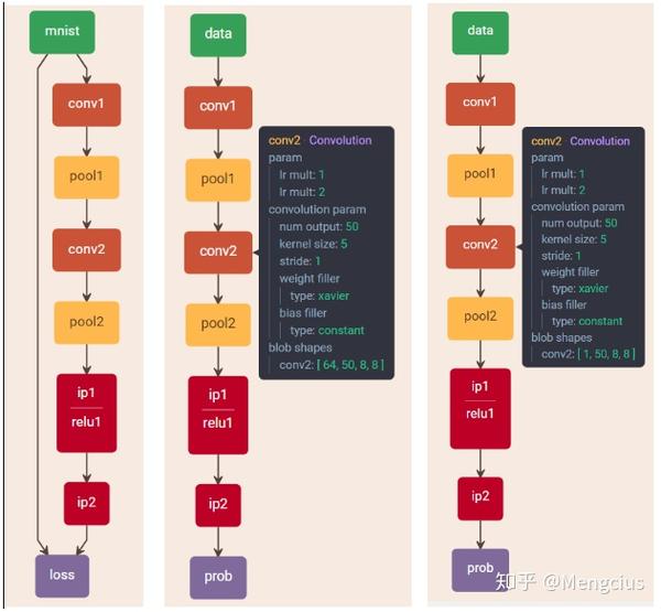
（3）可视化caffe网络结构

把caffe给的例程拷贝到网站 https://ethereon.github.io/netscope/#/editor 或 http://ethereon.github.io/netscope/#/editor，按shift+enter得到。

与最原始的相比，这里实现的LeNet加了relu，卷积核个数、全连接单元数也不一样，Sigmod也改为了softmax。如图左边的是训练和测试的lenet_train_test.prototxt，中间的是预测的lenet_depoly.prototxt（input_param { shape: { dim: 64 dim: 1 dim: 28 dim: 28 } } #64是batch_size），最右边的是lenet.prototxt（input_param { shape: { dim: 1 dim: 3 dim: 28 dim: 28 } } ）。

（4）训练
编写好lenet_solver.prototxt和lenet_train_test.prototxt后运行：

# coding utf-8
import caffe
caffe.set_device(0)  # GPU的设备号
caffe.set_mode_gpu() # gpu模式

solver = caffe.SGDSolver("./cnn_net/lenet/lenet_solver.prototxt")  # SGD，训练参数文件
solver.solve()

（5）预测结果
使用训练好的模型lenet_iter_10000.caffemodel，按照预测网络结构lenet.prototxt来推断。参考https://github.com/jklhj222/caffe_LeNet/blob/master/LeNet/caffe_test.py

#!/usr/bin/env python3
import os
import sys
import numpy as np
import matplotlib.pyplot as plt


caffe_root = '/home/s2c/pkg/local/caffe-master_cuDNN'


sys.path.insert(0, caffe_root + 'python') # Add the path of pycaffe into environment
import caffe


# Assign the structure of network, differ with lenet_train_test.prototxt
MODEL_FILE = '/home/s2c/pkg/local/caffe-master_cuDNN/examples/mnist/lenet.prototxt'
#MODEL_FILE = 'lenet_train_test.prototxt'
PRETRAINED = '/home/s2c/pkg/local/caffe-master_cuDNN/examples/mnist/lenet_iter_10000.caffemodel'


# lenet.prototxt, picture size (28x28）, black and white
IMAGE_FILE = '/home/s2c/pkg/local/caffe-master_cuDNN/examples/images/test4.png'


input_image = caffe.io.load_image(IMAGE_FILE, color=False)
net = caffe.Classifier(MODEL_FILE, PRETRAINED)
prediction = net.predict([input_image], oversample = False)
caffe.set_mode_gpu()
print( 'predicted class:', prediction[0].argmax() )
print( 'predicted class2:', prediction[0] )