天池_二手车交易价格预测数据分析

赛题数据链接 https://tianchi.aliyun.com/competition/entrance/231784/information

字典

Field	Description
SaleID	交易ID，唯一编码
name	汽车交易名称，已脱敏
regDate	汽车注册日期，例如20160101，2016年01月01日
model	车型编码，已脱敏
brand	汽车品牌，已脱敏
bodyType	车身类型：豪华轿车：0，微型车：1，厢型车：2，大巴车：3，敞篷车：4，双门汽车：5，商务车：6，搅拌车：7
fuelType	燃油类型：汽油：0，柴油：1，液化石油气：2，天然气：3，混合动力：4，其他：5，电动：6
gearbox	变速箱：手动：0，自动：1
power	发动机功率：范围 [ 0, 600 ]
kilometer	汽车已行驶公里，单位万km
notRepairedDamage	汽车有尚未修复的损坏：是：0，否：1
regionCode	地区编码，已脱敏
seller	销售方：个体：0，非个体：1
offerType	报价类型：提供：0，请求：1
creatDate	汽车上线时间，即开始售卖时间
price	二手车交易价格（预测目标）
v系列特征	匿名特征，包含v0-14在内15个匿名特征

step1：导入模块

## 基础工具
import numpy as np
import pandas as pd
import warnings
import matplotlib
import matplotlib.pyplot as plt
import seaborn as sns
from scipy.special import jn
from IPython.display import display, clear_output
import time

warnings.filterwarnings('ignore')
%matplotlib inline

## 模型预测的
from sklearn import linear_model
from sklearn import preprocessing
from sklearn.svm import SVR
from sklearn.ensemble import RandomForestRegressor,GradientBoostingRegressor

## 数据降维处理的
from sklearn.decomposition import PCA,FastICA,FactorAnalysis,SparsePCA

import lightgbm as lgb
import xgboost as xgb

## 参数搜索和评价的
from sklearn.model_selection import GridSearchCV,cross_val_score,StratifiedKFold,train_test_split
from sklearn.metrics import mean_squared_error, mean_absolute_error

step2：数据读取

#导入训练集和测试集
train_data =pd.read_csv('F:\python\天池_二手车交易价格预测\used_car_train_20200313.csv',sep=' ')
test_data=pd.read_csv('F:\python\天池_二手车交易价格预测\used_car_testB_20200421.csv',sep=' ')

1.数据量大小

## 输出数据的大小信息
print('Train data shape:',train_data.shape)
print('TestA data shape:',test_data.shape)

Train data shape: (150000, 31)
TestA data shape: (50000, 30)

2.数据浏览

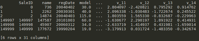
#前面三条数据+后面三条数据
train_data.head(3).append(train_data.tail(3))

 3.数据信息查看info()

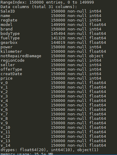
#info()可以查看特征类型，缺失情况
train_data.info()

4.查看列名

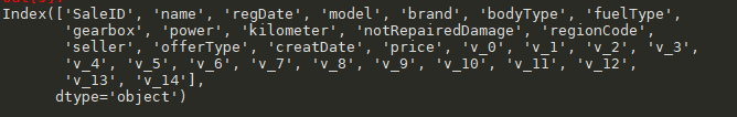
#通过.columns查看列名
train_data.columns

5.数据统计浏览

#.describe()
train_data.describe()

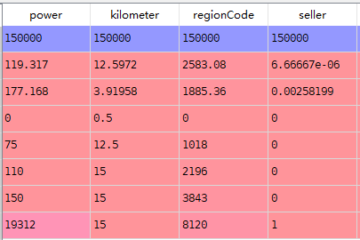
 剩下的不复制过来了

step3：缺失值

#查看每列缺失情况
train_data.isnull().sum()

#查看缺失占比情况
train_data.isnull().sum()/len(train_data)

#缺失值可视化
missing=train_data.isnull().sum()
missing[missing>0].sort_values().plot.bar()  #将大于0的拿出来并排序

 查看其他类型的空值，如‘-'’

#查看每个特征每个值的分布
for i in train_data.columns:
    print(train_data[i].value_counts())

发现notRepairedDamage：

#使用nan替代
train_data['notRepairedDamage'].replace('-',np.nan,inplace=True)

严重倾斜的数据，对因变量没有意义，可以删除

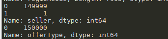
#删除特征
del train_data["seller"]
del train_data["offerType"]

step4：y值的分布

#y值的画图
plt.figure(1)
train_data['price'].plot.hist()
plt.figure(2)
sns.distplot(train_data['price'])

 

 价格不符合正态分布

step5：特征分析

1.区分类别特征和数字特征

#1.直接根据特征字段类型进行划分
#数据特征
numeric_features = train_data.select_dtypes(include=[np.number])
numeric_features.columns
#类别特征
categorical_features = train_data.select_dtypes(include=[np.object])
categorical_features.columns


#2.根据字典去分类,我们这次采用的是第二种
numeric_features = ['power', 'kilometer', 'v_0', 'v_1', 'v_2', 'v_3', 'v_4', 
                    'v_5', 'v_6', 'v_7', 'v_8', 'v_9', 'v_10', 'v_11', 'v_12', 'v_13','v_14' ]
categorical_features = ['name', 'model', 'brand', 'bodyType', 'fuelType', 
                        'gearbox', 'notRepairedDamage', 'regionCode',
                        'seller',    'offerType']

查看每个类别特征有多少个nunique分布

#nunique
for i in categorical_features:
    print(i+'特征分布如下:')
    print('{}特征有{}个不同的值'.format(i,train_data[i].nunique()))
    print(train_data[i].value_counts())

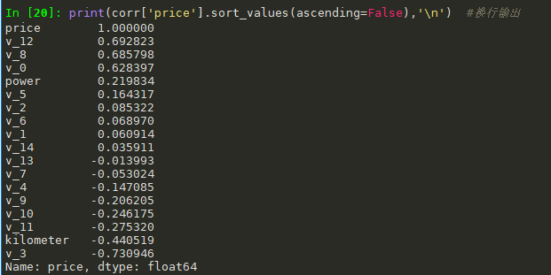
数据特征

#相关性分析
numeric_features.append('price')
corr=train_data[numeric_features].corr()
print(corr['price'].sort_values(ascending=False),'
')  #换行输出

 画地热图

sns.heatmap(corr)

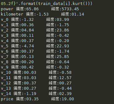
 查看数字特征的偏度和峰度

#查看偏度峰度

for i in numeric_features:
print('{}'.format(i),'偏度:{:05.2f}'.format(train_data[i].skew()),' ','峰度:{:05.2f}'.format(train_data[i].kurt()))

数字特征可视化

#方法一 
f=pd.melt(train_data,value_vars=numeric_features)
g=sns.FacetGrid(f,col='variable',col_wrap=2,sharex=False,sharey=False)
g=g.map(sns.distplot,'value')    

#方法二，不过这个画的图片 比较拥挤
for i,col in enumerate(numeric_features):
    plt.subplot(9,2,i+1)
    sns.distplot(train_data[col])

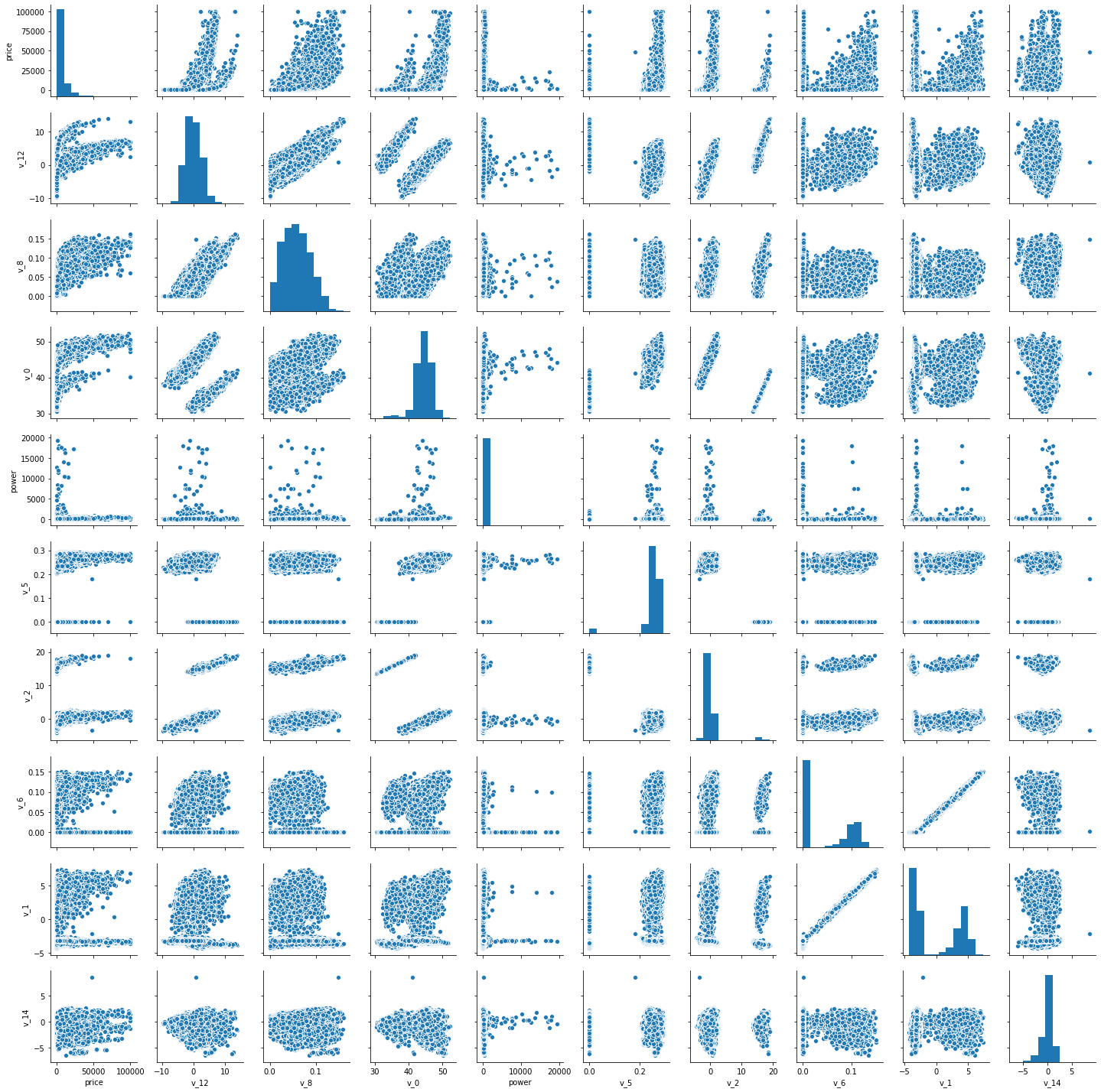
#查看数据特征相互关系
columns = ['price', 'v_12', 'v_8' , 'v_0', 'power', 'v_5',  'v_2', 'v_6', 'v_1', 'v_14']
sns.pairplot(train_data[columns],size=2)

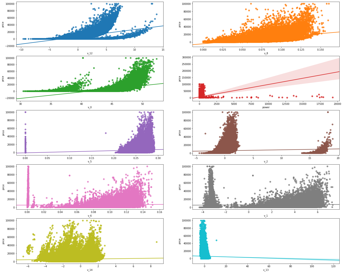
变量和y的回归关系可视化

fig,((ax1,ax2),(ax3,ax4),(ax5,ax6),(ax7,ax8),(ax9,ax10))=plt.subplots(
        nrows=5,ncols=2,figsize=(24,20))

v_12_plot=train_data[['v_12','price']]
sns.regplot(x='v_12',y='price',data=v_12_plot,ax=ax1)

v_8_plot=train_data[['v_8','price']]
sns.regplot(x='v_8',y='price',data=v_8_plot,ax=ax2)

v_0_plot=train_data[['v_0','price']]
sns.regplot(x='v_0',y='price',data=v_0_plot,ax=ax3)

power_plot=train_data[['power','price']]
sns.regplot(x='power',y='price',data=power_plot,ax=ax4)

v_5_plot=train_data[['v_5','price']]
sns.regplot(x='v_5',y='price',data=v_5_plot,ax=ax5)

v_2_plot=train_data[['v_2','price']]
sns.regplot(x='v_2',y='price',data=v_2_plot,ax=ax6)

v_6_plot=train_data[['v_6','price']]
sns.regplot(x='v_6',y='price',data=v_6_plot,ax=ax7)

v_1_plot=train_data[['v_1','price']]
sns.regplot(x='v_1',y='price',data=v_1_plot,ax=ax8)

v_14_plot=train_data[['v_14','price']]
sns.regplot(x='v_14',y='price',data=v_14_plot,ax=ax9)

v_13_plot=train_data[['v_13','price']]
sns.regplot(x='v_13',y='price',data=v_13_plot,ax=ax10)

#类别特征的nunique分布
for i in categorical_features:
    print('{}: 有 {} 个不重复的值'.format(i,train_data[i].nunique()))

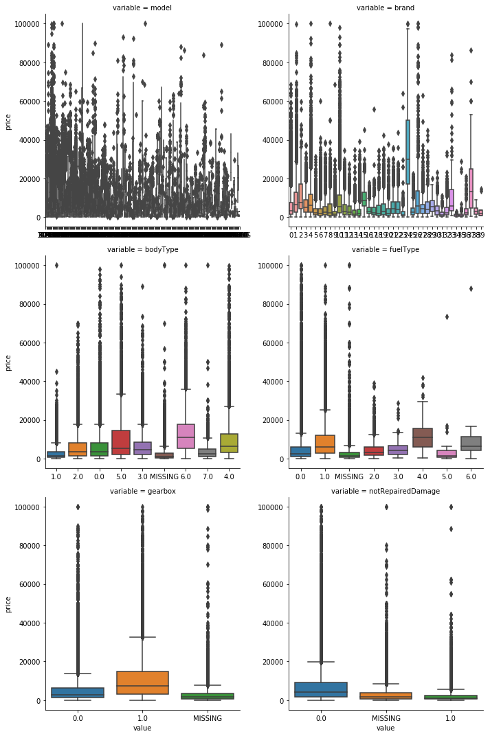
 类别特征可视化

#类别特征画箱型图
#由上面的nunique()可见name和regionCode的值太多，不宜做图，以此将这2个去掉
cols=['model',
 'brand',
 'bodyType',
 'fuelType',
 'gearbox',
 'notRepairedDamage']

for i in cols:
    train_data[i]=train_data[i].astype('category')  #将数据类型变成类别型
    if train_data[i].isnull().any():
        train_data[i]=train_data[i].cat.add_categories(['MISSING'])
        train_data[i]=train_data[i].fillna('MISSING')
    
    
def boxplot(x,y,**kwargs):
    sns.boxplot(x=x,y=y)

f=pd.melt(train_data,id_vars=['price'],value_vars=cols)
g=sns.FacetGrid(f,col='variable',col_wrap=2, sharex=False, sharey=False, size=5)
g.map(boxplot,'value','price')

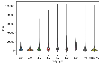
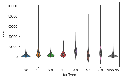
#画小提琴图
for i in cols:
    sns.violinplot(x=i,y='price',data=train_data)
    plt.show()  #很奇怪，如果没有这个语句就只有一张图片，有了就会继续for循环

 

 

 

 

 

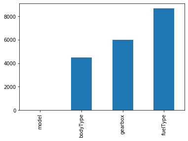
categorical_features = ['model',
 'brand',
 'bodyType',
 'fuelType',
 'gearbox',
 'notRepairedDamage']


#类别特征的类别个数和y值的柱状图
def bar_plot(x,y,**kwargs):
    sns.barplot(x=x,y=y)
    x=plt.xticks(rotation=90)

f = pd.melt(train_data, id_vars=['price'], value_vars=categorical_features)
g = sns.FacetGrid(f, col="variable",  col_wrap=2, sharex=False, sharey=False, size=5)
g = g.map(bar_plot, "value", "price")

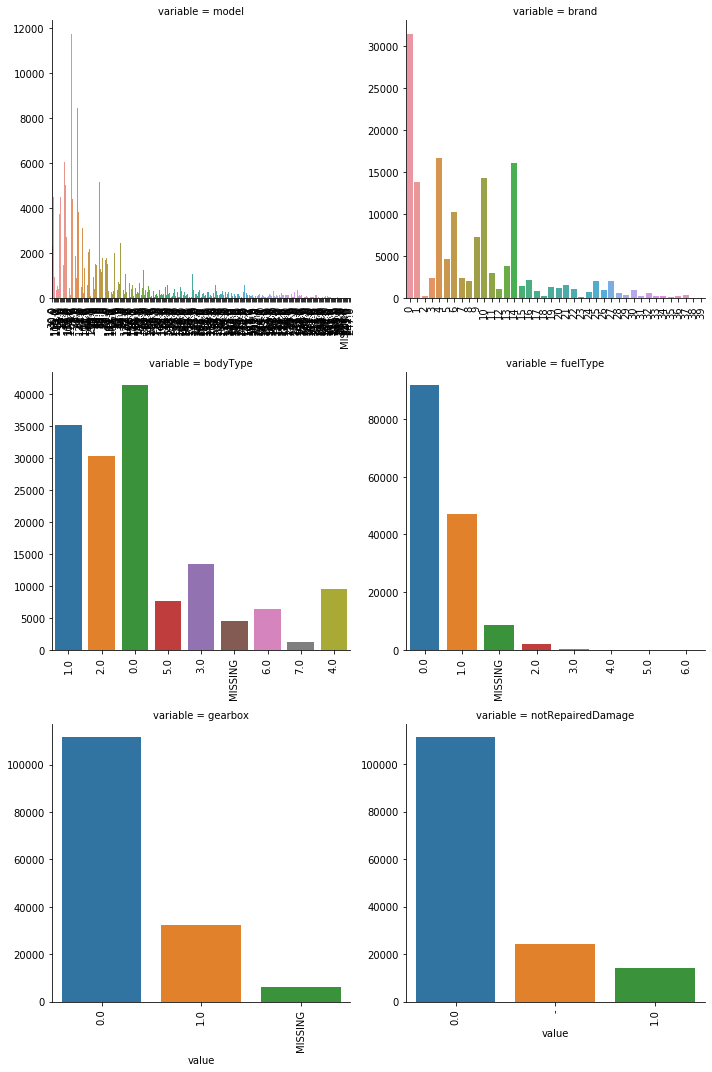
#类别特征的每个类别频数可视化(count_plot)
def count_plot(x,  **kwargs):
    sns.countplot(x=x)
    x=plt.xticks(rotation=90)

f = pd.melt(train_data,  value_vars=categorical_features)
g = sns.FacetGrid(f, col="variable",  col_wrap=2, sharex=False, sharey=False, size=5)
g = g.map(count_plot, "value")