1.1 工具变量法
OLS 有一个经典的假设:解释变量与随机误差项不相关,即 。如果存在解释变量违背了这个假设,则估计出的参数是有偏的,也是不一致的。
工具变量 (IV) 法为解决「内生解释变量」问题提供了一种可行的方法。为此,我们需要找到满足以下条件的「外生解释变量 (z)」:
- 与内生解释变量相关,即
- 与随机误差项不相关,即
根据「内生解释变量」与「工具变量」间的数量关系,又可以分为以下几种情况:
- 不可识别 (unidentified):工具变量数小于内生解释变量数;
- 恰好识别 (just or exactly indentified):工具变量数等于内生解释变量数;
- 过度识别 (overindentified):工具变量数大于内生解释变量数。
在「恰好识别」的情况下,我们可以估计 ,而在「过度识别」的情况下,则需要通过两阶段最小二乘法 (Two Stage Least Square,2SLS 或 TSLS) 估计 。当然在「恰好识别」的情况下,我们也可以用 2SLS 进行估计。但是,在「不可识别」情况下,以上方法失效。2SLS 主要通过以下两阶段实现:
- 第一阶段,用内生解释变量对工具变量回归;
- 第二阶段,用被解释变量对第一阶段回归的拟合值回归。
值得注意, 2SLS 只有在「同方差」的情况下才是最优效率的,而在「过度识别」和「异方差」的情况下,广义矩估计 (Generalized Method of Moments, GMM) 才是最有效率的。关于 GMM 介绍详见:「Stata:GMM 简介及实现范例」和「GMM 简介与 Stata 实现」。
在使用工具变量之前,我们仍需进行若干检验:
- 解释变量内生性的检验;
- 弱工具变量检验;
- 过度识别检验。
在「恰好识别」的情况下,我们无法检验工具变量的外生性,只能进行「定性讨论或依赖专家意见」,详见「IV-估计:工具变量不外生时也可以用!」。因此,我们重点关注「过度识别检验」的方法和在 Stata 中实现。
1.2 两阶段最小二乘法
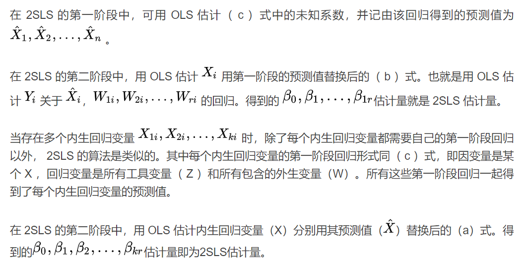
两阶段最小二乘法其本质上是属于工具变量,回归分两个阶段进行,因此而得名。具体机理是:
第一步,将结构方程先转换为简化式模型(约简型方程),简化式模型里的每一个方程都不存在随机解释变量问题,可以直接采用普通最小二乘法进行估计。
第二步,由第一步得出的估计量替换 Y 。该方程中不存在随机解释变量问题,也可以直接用普通最小二乘法进行估计。
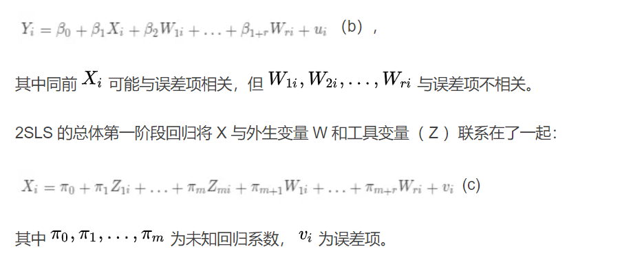
例子:一般 IV 回归模型为:
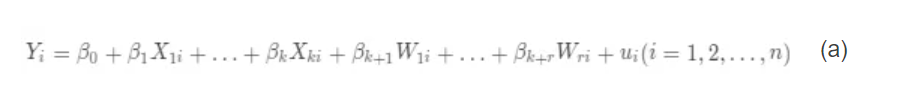
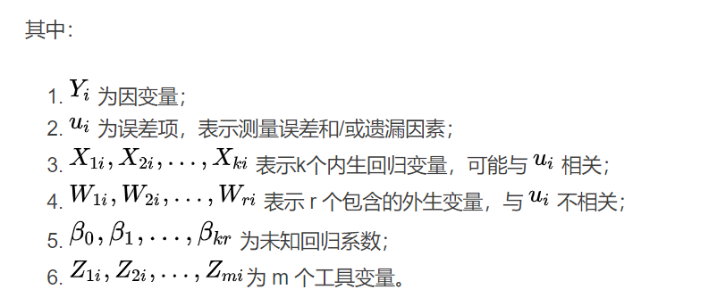
以单内生回归变量的 2SLS 为例,当只有一个内生回归变量 X 和一些其他的包含的外生变量时,感兴趣的方程为:
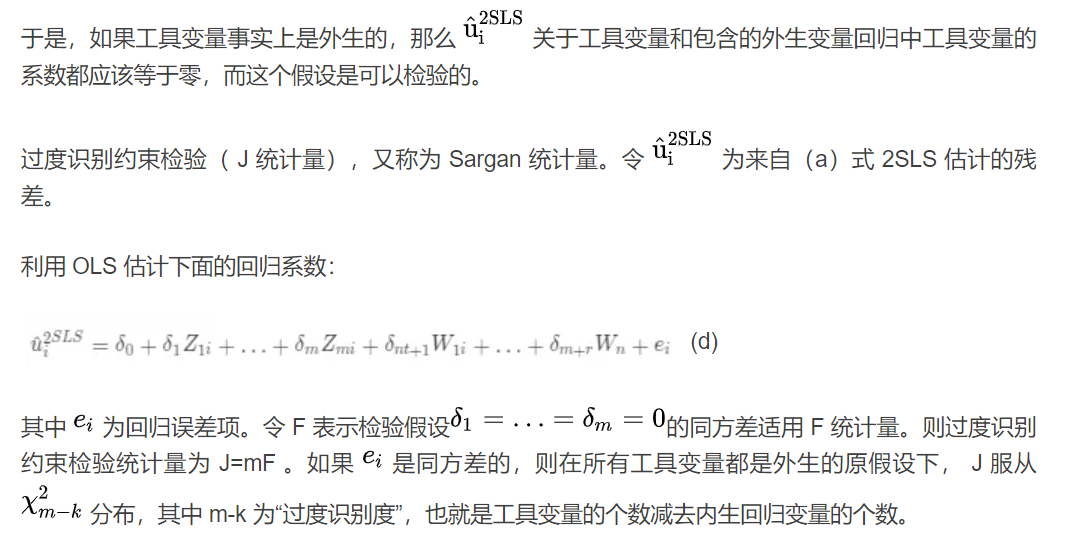
2. 过度识别检验
2.1过度识别检验原理
上面提到了,只有恰好识别和过度识别才能用 IV 方法估计。假设待估参数的个数为 k ,矩条件的个数为 l 。当 k=l 时,称为“恰好识别”,当 k<l 时,称为="过度识别"。
一个很重要的命题是:只有过度识别情况下才能检验工具变量的外生性,而恰好识别情况下无法检验。
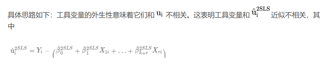
为基于所有工具变量的 2SLS 回归估计残差(由于抽样变异性因此是近似的而不是精确地,注意到这些残差是利用 X 值而不是用其第一阶段的预测值得到的。)
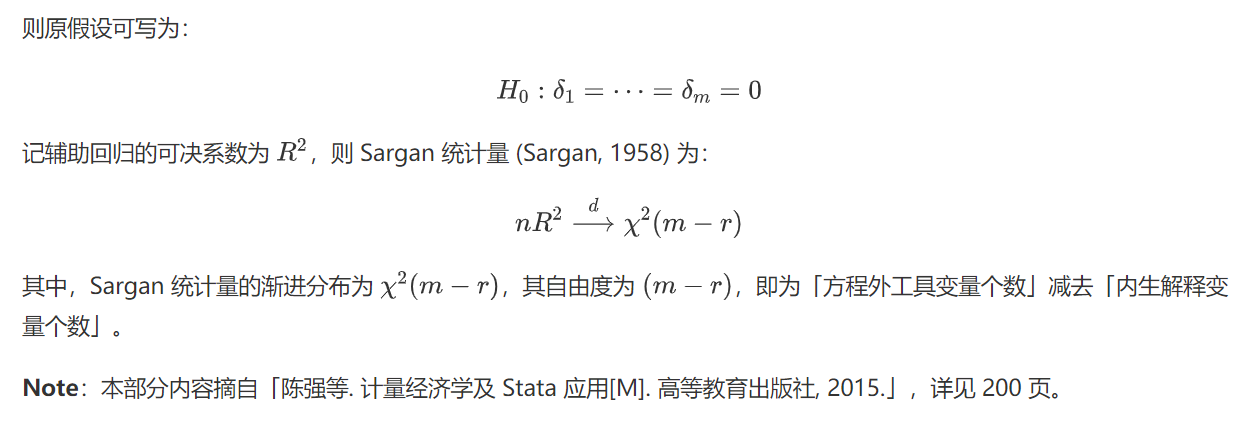
2.2.1 Sargan 检验

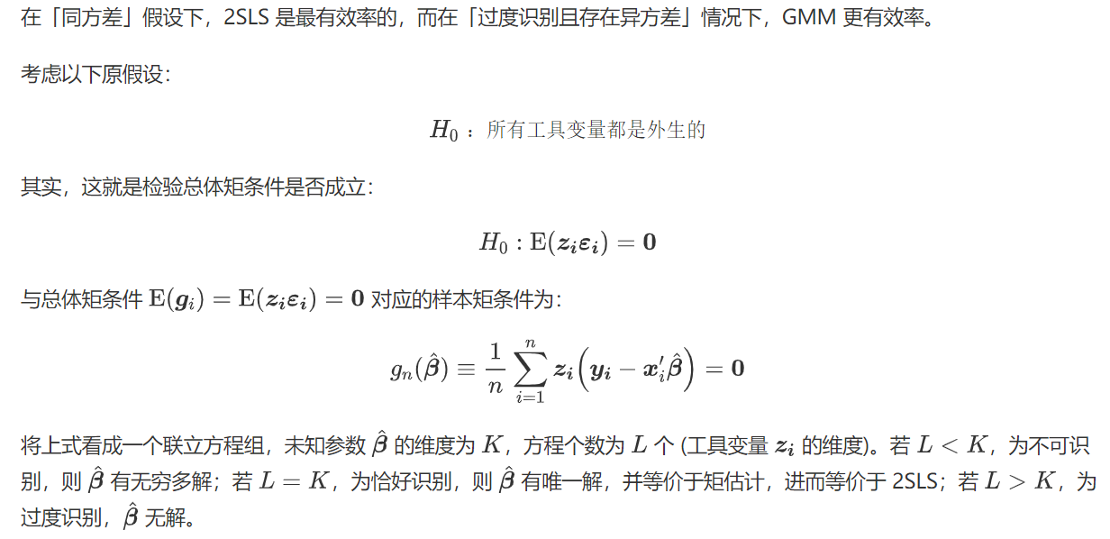
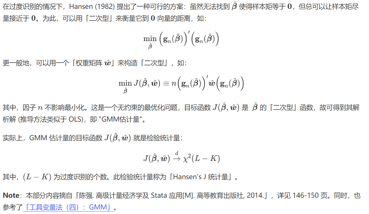
2.2.2 Hansen J 检验
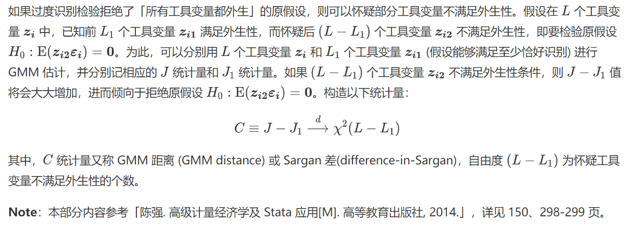
2.2.3 C 统计量
3. 过度识别检验的 Stata 实现
3.1 ivreg2 命令
以官方 griliches76.dta 数据为例,lw 为工资对数,s 为受教育年限,expr 为工龄,tenure 为现单位工作年数,rns 为美国南方虚拟变量 (住在南方 = 1),smsa 为大城市虚拟变量 (住在大城市 = 1),iq 为智商,med 为母亲受教育年限,kww 为一项职业测试成绩 (score on knowledge in world of work test),age 为年龄,mrt 为婚姻状况 (已婚 = 1)。
在研究「智商」对「工资」的影响时,「智商」通常会被认为是一个内生的解释变量,因此我们需要为「智商」寻找工具变量。当然外生解释变量可以被看作自身的工具变量。在这里,我们将母亲受教育年限 (med)、职业测试成绩 (kww)、年龄 (age) 和婚姻状况 (mrt)作为「智商」的工具变量,并进行「过度识别」检验。
在使用 ivreg2 命令进行工具变量回归时,默认提供 Sargan 统计量,而在命令后加入 robust、bw、cluster 等选项时,Stata 默认提供 Hansen J 统计量。若要报告 统计量,只需在命令后加入 orthog(varlist_ex) 选项,其中 varlist_ex 为需要检验外生性的变量。关于 ivreg2 更多介绍,详见 help ivreg2。
*-安装命令
  ssc install ivreg2, replace

*-Sargan 检验
  use http://fmwww.bc.edu/ec-p/data/hayashi/griliches76.dta
  ivreg2 lw s expr tenure rns smsa i.year (iq=med kww age mrt)

*-Hansen J 检验
  ivreg2 lw s expr tenure rns smsa i.year (iq=med kww age mrt), robust

*-C 统计量
  ivreg2 lw s expr tenure rns smsa i.year (iq=med kww age mrt), orthog(s)
.   ivreg2 lw s expr tenure rns smsa i.year (iq=med kww age mrt)

IV (2SLS) estimation
--------------------

Estimates efficient for homoskedasticity only
Statistics consistent for homoskedasticity only

                                                      Number of obs =      758
                                                      F( 12,   745) =    45.91
                                                      Prob > F      =   0.0000
Total (centered) SS     =  139.2861498                Centered R2   =   0.4255
Total (uncentered) SS   =  24652.24662                Uncentered R2 =   0.9968
Residual SS             =   80.0182337                Root MSE      =    .3249

------------------------------------------------------------------------------
          lw |      Coef.   Std. Err.      z    P>|z|     [95% Conf. Interval]
-------------+----------------------------------------------------------------
          iq |   .0001747   .0039035     0.04   0.964     -.007476    .0078253
           s |   .0691759   .0129366     5.35   0.000     .0438206    .0945312
        expr |    .029866   .0066393     4.50   0.000     .0168533    .0428788
      tenure |   .0432738   .0076271     5.67   0.000     .0283249    .0582226
         rns |  -.1035897    .029481    -3.51   0.000    -.1613715   -.0458079
        smsa |   .1351148   .0266573     5.07   0.000     .0828674    .1873623
             |
        year |
         67  |   -.052598   .0476924    -1.10   0.270    -.1460734    .0408774
         68  |   .0794686   .0447194     1.78   0.076    -.0081797    .1671169
         69  |   .2108962   .0439336     4.80   0.000     .1247878    .2970045
         70  |   .2386338   .0509733     4.68   0.000     .1387281    .3385396
         71  |   .2284609   .0437436     5.22   0.000     .1427251    .3141967
         73  |   .3258944   .0407181     8.00   0.000     .2460884    .4057004
             |
       _cons |    4.39955   .2685443    16.38   0.000     3.873213    4.925887
------------------------------------------------------------------------------
Underidentification test (Anderson canon. corr. LM statistic):          52.436
                                                   Chi-sq(4) P-val =    0.0000
------------------------------------------------------------------------------
Weak identification test (Cragg-Donald Wald F statistic):               13.786
Stock-Yogo weak ID test critical values:  5% maximal IV relative bias    16.85
                                         10% maximal IV relative bias    10.27
                                         20% maximal IV relative bias     6.71
                                         30% maximal IV relative bias     5.34
                                         10% maximal IV size             24.58
                                         15% maximal IV size             13.96
                                         20% maximal IV size             10.26
                                         25% maximal IV size              8.31
Source: Stock-Yogo (2005).  Reproduced by permission.
------------------------------------------------------------------------------
Sargan statistic (overidentification test of all instruments):          87.655
                                                   Chi-sq(3) P-val =    0.0000
------------------------------------------------------------------------------
Instrumented:         iq
Included instruments: s expr tenure rns smsa 67.year 68.year 69.year 70.year
                      71.year 73.year
Excluded instruments: med kww age mrt
------------------------------------------------------------------------------
 *-Hansen J 检验
.   ivreg2 lw s expr tenure rns smsa i.year (iq=med kww age mrt), robust

IV (2SLS) estimation
--------------------

Estimates efficient for homoskedasticity only
Statistics robust to heteroskedasticity

                                                      Number of obs =      758
                                                      F( 12,   745) =    46.94
                                                      Prob > F      =   0.0000
Total (centered) SS     =  139.2861498                Centered R2   =   0.4255
Total (uncentered) SS   =  24652.24662                Uncentered R2 =   0.9968
Residual SS             =   80.0182337                Root MSE      =    .3249

------------------------------------------------------------------------------
             |               Robust
          lw |      Coef.   Std. Err.      z    P>|z|     [95% Conf. Interval]
-------------+----------------------------------------------------------------
          iq |   .0001747   .0041241     0.04   0.966    -.0079085    .0082578
           s |   .0691759   .0132907     5.20   0.000     .0431266    .0952253
        expr |    .029866   .0066974     4.46   0.000     .0167394    .0429926
      tenure |   .0432738   .0073857     5.86   0.000     .0287981    .0577494
         rns |  -.1035897    .029748    -3.48   0.000    -.1618947   -.0452847
        smsa |   .1351148    .026333     5.13   0.000     .0835032    .1867265
             |
        year |
         67  |   -.052598   .0457261    -1.15   0.250    -.1422195    .0370235
         68  |   .0794686   .0428231     1.86   0.063    -.0044631    .1634003
         69  |   .2108962   .0408774     5.16   0.000     .1307779    .2910144
         70  |   .2386338   .0529825     4.50   0.000     .1347901    .3424776
         71  |   .2284609   .0426054     5.36   0.000     .1449558     .311966
         73  |   .3258944   .0405569     8.04   0.000     .2464044    .4053844
             |
       _cons |    4.39955    .290085    15.17   0.000     3.830994    4.968106
------------------------------------------------------------------------------
Underidentification test (Kleibergen-Paap rk LM statistic):             41.537
                                                   Chi-sq(4) P-val =    0.0000
------------------------------------------------------------------------------
Weak identification test (Cragg-Donald Wald F statistic):               13.786
                         (Kleibergen-Paap rk Wald F statistic):         12.167
Stock-Yogo weak ID test critical values:  5% maximal IV relative bias    16.85
                                         10% maximal IV relative bias    10.27
                                         20% maximal IV relative bias     6.71
                                         30% maximal IV relative bias     5.34
                                         10% maximal IV size             24.58
                                         15% maximal IV size             13.96
                                         20% maximal IV size             10.26
                                         25% maximal IV size              8.31
Source: Stock-Yogo (2005).  Reproduced by permission.
NB: Critical values are for Cragg-Donald F statistic and i.i.d. errors.
------------------------------------------------------------------------------
Hansen J statistic (overidentification test of all instruments):        74.165
                                                   Chi-sq(3) P-val =    0.0000
------------------------------------------------------------------------------
Instrumented:         iq
Included instruments: s expr tenure rns smsa 67.year 68.year 69.year 70.year
                      71.year 73.year
Excluded instruments: med kww age mrt
------------------------------------------------------------------------------
. *-C 统计量
.   ivreg2 lw s expr tenure rns smsa i.year (iq=med kww age mrt), orthog(age)

IV (2SLS) estimation
--------------------

Estimates efficient for homoskedasticity only
Statistics consistent for homoskedasticity only

                                                      Number of obs =      758
                                                      F( 12,   745) =    45.91
                                                      Prob > F      =   0.0000
Total (centered) SS     =  139.2861498                Centered R2   =   0.4255
Total (uncentered) SS   =  24652.24662                Uncentered R2 =   0.9968
Residual SS             =   80.0182337                Root MSE      =    .3249

------------------------------------------------------------------------------
          lw |      Coef.   Std. Err.      z    P>|z|     [95% Conf. Interval]
-------------+----------------------------------------------------------------
          iq |   .0001747   .0039035     0.04   0.964     -.007476    .0078253
           s |   .0691759   .0129366     5.35   0.000     .0438206    .0945312
        expr |    .029866   .0066393     4.50   0.000     .0168533    .0428788
      tenure |   .0432738   .0076271     5.67   0.000     .0283249    .0582226
         rns |  -.1035897    .029481    -3.51   0.000    -.1613715   -.0458079
        smsa |   .1351148   .0266573     5.07   0.000     .0828674    .1873623
             |
        year |
         67  |   -.052598   .0476924    -1.10   0.270    -.1460734    .0408774
         68  |   .0794686   .0447194     1.78   0.076    -.0081797    .1671169
         69  |   .2108962   .0439336     4.80   0.000     .1247878    .2970045
         70  |   .2386338   .0509733     4.68   0.000     .1387281    .3385396
         71  |   .2284609   .0437436     5.22   0.000     .1427251    .3141967
         73  |   .3258944   .0407181     8.00   0.000     .2460884    .4057004
             |
       _cons |    4.39955   .2685443    16.38   0.000     3.873213    4.925887
------------------------------------------------------------------------------
Underidentification test (Anderson canon. corr. LM statistic):          52.436
                                                   Chi-sq(4) P-val =    0.0000
------------------------------------------------------------------------------
Weak identification test (Cragg-Donald Wald F statistic):               13.786
Stock-Yogo weak ID test critical values:  5% maximal IV relative bias    16.85
                                         10% maximal IV relative bias    10.27
                                         20% maximal IV relative bias     6.71
                                         30% maximal IV relative bias     5.34
                                         10% maximal IV size             24.58
                                         15% maximal IV size             13.96
                                         20% maximal IV size             10.26
                                         25% maximal IV size              8.31
Source: Stock-Yogo (2005).  Reproduced by permission.
------------------------------------------------------------------------------
Sargan statistic (overidentification test of all instruments):          87.655
                                                   Chi-sq(3) P-val =    0.0000
-orthog- option:
Sargan statistic (eqn. excluding suspect orthogonality conditions):     47.413
                                                   Chi-sq(2) P-val =    0.0000
C statistic (exogeneity/orthogonality of suspect instruments):          40.242
                                                   Chi-sq(1) P-val =    0.0000
Instruments tested:   age
------------------------------------------------------------------------------
Instrumented:         iq
Included instruments: s expr tenure rns smsa 67.year 68.year 69.year 70.year
                      71.year 73.year
Excluded instruments: med kww age mrt
------------------------------------------------------------------------------
可以看出,无论是「Sargan 检验」还是「Hansen J」检验都拒绝了「原假设:所有工具变量都外生」,表明存在一部分内生的工具变量。进一步,我们又构造了 统计量来检验工具变量 age 的外生性,检验结果显著拒绝了「原假设:工具变量 age 是外生的」。
3.2GMM 中过度识别的命令为 estat overid
若是 Sargen - Baseman 检验的统计量对应的 p 值大于 0.05 ,则认为所有的工具变量都是外生的,也就是有效的,反之则是无效的。(原假设是所有工具变量是外省的,若是 p 值小于 0.05 ,则拒绝原假设)
sysuse auto,clear
ivregress gmm mpg gear_ratio (turn =weight length headroom),wmatrix(robust) small
estat overid
过度识别检验( Sargen - Baseman 检验)的结果为:
Test of overidentifying restriction:
Hansen's J chi2(2) =  .54848 (p = 0.7601)
根据结果可知, Sargen - Baseman 检验统计量对应的 p 值大于 0.05 ,所有的工具变量都是外生有效的。
3.3 xtbond2 命令
以 mus08psidextract.dta 为例,该数据包含 595 名美国人 1976-1982 与工资相关的变量 (n = 595, T = 7),其中 lwage 为工资对数,wks 为工作周数,ms 为婚否,union 为是否由工会合同确定工资,occ 为是否是蓝领工人,south 为是否在美国南部,smsa 为是否住在大城市,ind 为是否在在制造业工作。
在使用 xtabond2 命令进行 GMM 回归时,Stata 同时提供 Sargan 检验、Hansen J 检验、以及 统计量。关于 Sargan 检验 和 Hansen J 检验,一般认为 Hansen J 检验结果更为稳健。
*-安装命令
  ssc install xtabond2, replace

*-动态面板过度识别检验
  sysuse mus08psidextract.dta, clear
  xtabond2 lwage L(1/2).lwage L(0/1).wks ms union occ south smsa ind, \
           gmm(lwage, lag(2 4)) gmm(wks ms union, lag(2 3))  \
           iv(occ south smsa ind) nolevel twostep robust
上述命令中,L(1/2).lwage 表示 L1.wage L2.wage,L(0/1).wks 表示 wks L1.wks;gmm(lwage, lag(2 4)) 表示使用 lwage 的 2-4 阶作为 GMM 式工具变量,gmm(wks ms union, lag(2 3)) 表示使用 wks ms union 的 2-3 阶作为 GMM 式工具变量,iv(occ south smsa ind) 表示使用 occ south smsa ind 作为自身工具变量。
Dynamic panel-data estimation, two-step difference GMM
------------------------------------------------------------------------------
Group variable: id                              Number of obs      =      2380
Time variable : t                               Number of groups   =       595
Number of instruments = 39                      Obs per group: min =         4
Wald chi2(10) =   1287.77                                      avg =      4.00
Prob > chi2   =     0.000                                      max =         4
------------------------------------------------------------------------------
             |              Corrected
       lwage |      Coef.   Std. Err.      z    P>|z|     [95% Conf. Interval]
-------------+----------------------------------------------------------------
       lwage |
         L1. |    .611753   .0373491    16.38   0.000     .5385501    .6849559
         L2. |   .2409058   .0319939     7.53   0.000     .1781989    .3036127
             |
         wks |
         --. |  -.0159751   .0082523    -1.94   0.053    -.0321493     .000199
         L1. |   .0039944   .0027425     1.46   0.145    -.0013807    .0093695
             |
          ms |   .1859324    .144458     1.29   0.198       -.0972    .4690649
       union |  -.1531329   .1677842    -0.91   0.361    -.4819839    .1757181
         occ |  -.0357509   .0347705    -1.03   0.304    -.1038999     .032398
       south |  -.0250368   .2150806    -0.12   0.907     -.446587    .3965134
        smsa |  -.0848223   .0525243    -1.61   0.106     -.187768    .0181235
         ind |   .0227008   .0424207     0.54   0.593    -.0604422    .1058437
------------------------------------------------------------------------------
Instruments for first differences equation
  Standard
    D.(occ south smsa ind)
  GMM-type (missing=0, separate instruments for each period unless collapsed)
    L(2/3).(wks ms union)
    L(2/4).lwage
------------------------------------------------------------------------------
Arellano-Bond test for AR(1) in first differences: z =  -4.52  Pr > z =  0.000
Arellano-Bond test for AR(2) in first differences: z =  -1.60  Pr > z =  0.109
------------------------------------------------------------------------------
Sargan test of overid. restrictions: chi2(29)   =  59.55  Prob > chi2 =  0.001
  (Not robust, but not weakened by many instruments.)
Hansen test of overid. restrictions: chi2(29)   =  39.88  Prob > chi2 =  0.086
  (Robust, but weakened by many instruments.)

Difference-in-Hansen tests of exogeneity of instrument subsets:
  gmm(lwage, lag(2 4))
    Hansen test excluding group:     chi2(18)   =  23.59  Prob > chi2 =  0.169
    Difference (null H = exogenous): chi2(11)   =  16.29  Prob > chi2 =  0.131
  gmm(wks ms union, lag(2 3))
    Hansen test excluding group:     chi2(5)    =   6.43  Prob > chi2 =  0.266
    Difference (null H = exogenous): chi2(24)   =  33.44  Prob > chi2 =  0.095
  iv(occ south smsa ind)
    Hansen test excluding group:     chi2(25)   =  28.00  Prob > chi2 =  0.308
    Difference (null H = exogenous): chi2(4)    =  11.87  Prob > chi2 =  0.018
可以看出,工具变量总的个数为 39,而内生变量的个数为 10。同时,扰动项的差分存在一阶自相关,而不存在二阶自相关,故不能拒绝原假设「扰动项无自相关」,可以使用差分 GMM。
Sargan 统计量和 Hansen 统计量在 10% 的水平上都拒绝了「所有工具变量都外生」的原假设。值得注意的是,Sargan 统计量并不稳健,但不受工具变量过多的影响,而 Hansen 统计量虽然稳健,但受工具变量过多的影响。

4. 过度识别检验统计量无法计算
4.1 原因
在使用 ivreg2 命令进行估计时,我们经常会发现 Sargan 检验或 Hansen J 检验始终无法通过。这可能是由于「工具变量过多」造成的,如模型中控制了年份固定效应、地区固定效应和行业固定效应等虚拟变量。
但是,当「虚拟变量的个数 < (外生变量个数 + 工具变量个数)」时,正交条件对应的方差-协方差矩阵 有可能是非满秩矩阵,此时我们无法计算出 矩阵的逆矩阵 ,从而导致过度识别检验的统计量无法计算。更为详细的介绍,可通过 help ivreg2 查看。
4.2 解决方法
利用 Frisch-Waugh-Lovell (FWL) 定理,我们可以尝试「partial out」一定数量的外生变量 (通常主要是虚拟变量),以保证 矩阵满秩。在使用 ivreg2 命令执行 2SLS 或 GMM 估计时,我们可以加入 partial() 选项,选项中先填入所有外生的虚拟变量,如有必要,可以进一步加入其它外生的解释变量。
4.3 Stata 实现
接下来,以案例形式简要介绍「partial out」的原理。
范例 1:partial out 连续变量
sysuse "auto.dta", clear
    rename (price length weight) (Y X1 X2)

    ivregress 2sls Y X1 X2
    est store m0  //原始结果

    *-Partial out X2
    ivregress 2sls Y X2      //从 y  中除去 X2 的影响
    predict e_y, res

    ivregress 2sls X1 X2     //从 X1 中除去 X2 的影响
    predict e_x1, res

    ivregress 2sls e_y e_x1  //partial out 后的的回归结果
    est store m1

    esttab m0 m1, nogap
    restore
 --------------------------------------------
                          (1)             (2)
                            Y             e_y
    --------------------------------------------
    X1                 -97.96*
                      (-2.55)
    X2                  4.699***
                       (4.27)
    e_x1                               -97.96*
                                      (-2.55)
    _cons             10386.5*       2.04e-12
                       (2.46)          (0.00)
    --------------------------------------------
    N                      74              74
    --------------------------------------------
    t statistics in parentheses
    * p<0.05, ** p<0.01, *** p<0.001

    *-Notes:
    (1) 如果采用 regress 进行回归,SE 会有微小差异,
        主要是因为 regress 会针对小样本进行自由度调整。
    (2) 采用 IV/GMM 估计,即 ivregress 命令就不会有这个问题了。
范例 2:partial out 虚拟变量
sysuse auto, clear
  drop if rep78==.
  global yx "price wei len mpg"

  ivregress 2sls $yx i.rep78
  est store m0

  bysort rep78: center $yx, inplace //prefix(c_)
  ivregress 2sls $yx
  est store m1

  esttab m0 m1, nogap nobase
  restore
  --------------------------------------------
                            (1)             (2)
                          price           price
      --------------------------------------------
      weight              5.187***        5.187***
                         (4.74)          (4.74)
      length             -124.2***       -124.2***
                        (-3.29)         (-3.29)
      mpg                -126.8          -126.8
                        (-1.60)         (-1.60)
      2.rep78            1137.3
                         (0.67)
      3.rep78            1254.6
                         (0.80)
      4.rep78            2267.2
                         (1.42)
      5.rep78            3850.8*
                         (2.29)
      _cons             14614.5*      0.0000116
                         (2.52)          (0.00)
      --------------------------------------------
      N                      69              69
      --------------------------------------------
      t statistics in parentheses
      * p<0.05, ** p<0.01, *** p<0.001

     *-Note: FE 模型其实就是先 partial out 公司虚拟变量,然后再对转换后的数据执行 OLS 回归。
范例 3:是否加入 partial() 选项无影响
*-数据下载地址
* https://gitee.com/arlionn/data/blob/master/data01/Acem_data_done.dta

  use Acem_data_done.dta, clear
  global y "change_gdp"
  global x "change_dependency"
  global z "devo1990 lpop1990 base_dependency" // 控制变量
  global IVs "birthrate1960_1965 birthrate1965_1970 birthrate1970_1975 birthrate1975_1980 birthrate1980_1985 birthrate1985_1990"// 工具变量

  ivregress 2sls $y ($x=$IVs) $z i.region_code, robust  //官方命令
    est store a1

    ivreg2 $y ($x=$IVs) $z i.region_code, robust    // 等价-外部命令
    est store a2   // without -partial()- option

  ivreg2 $y ($x=$IVs) $z i.region_code, robust ///
  partial(lpop1990 i.region_code base_dependency)
  est store c5   // with -partial()- option

*-手动计算:(特别注意:此时的 SE 是错误的!)
* Step1:
    reg $x $IVs $z i.region_code
    cap drop xhat
    predict xhat

* Step2:
    reg $y xhat $z i.region_code
    est store a3

*-对比结果:
  local m "a1 a2 c5 a3"
  esttab `m' `s', nogap  replace        ///
  b(%6.3f) s(N r2_a rkf j jp)    ///
  star(* 0.1 ** 0.05 *** 0.01)   ///
  order(change_dependency xhat)  ///
  indicate("Region Dummies =*.region_code")  ///
  addnotes("*** 1% ** 5% * 10%") nobase

----------------------------------------------------------------------------
                   (a1)            (a2)             (c5)            (a3)
                no-parital      no-partial       partial-out       by-hand
CMD             ivregress         ivreg2          ivreg2          regress
----------------------------------------------------------------------------
change_dep~y        1.703***        1.703***        1.703***
                   (4.14)          (4.14)          (4.14)
xhat                                                                1.703***
                                                                   (3.80)
devo1990           -0.190***       -0.190***       -0.190***       -0.190***
                  (-4.22)         (-4.22)         (-4.22)         (-4.58)
lpop1990           -0.017          -0.017                          -0.017
                  (-0.83)         (-0.83)                         (-0.96)
base_depen~y       -0.041          -0.041                          -0.041
                  (-0.14)         (-0.14)                         (-0.13)
_cons               1.899***        1.899***                        1.899***
                   (4.99)          (4.99)                          (5.54)
Region Dum~s          Yes             Yes              No             Yes
----------------------------------------------------------------------------
N                 169.000         169.000         169.000         169.000
r2_a                0.179           0.179          -0.024           0.261
rkf                                19.365          19.365
j                                   4.280           4.280
jp                                  0.510           0.510
----------------------------------------------------------------------------
t statistics in parentheses, p<0.1, ** p<0.05, *** p<0.01
Notes:(1) a1 与 c5 结果完全相同,因此 partial out 部分变量不影响系数估计值;(2) partial out 的目的是为了减少干扰项的方差协方差矩阵 的维度,以便合理计算 Sargan 和 Hansen J 统计量。
范例4:是否加入 partial 选项有显著影响
我们将通过下例来演示加入 partial 选项引起的变化。
use http://fmwww.bc.edu/ec-p/data/hayashi/griliches76.dta, clear
ivreg2 lw s expr tenure rns smsa i.year (iq=med kww age), cluster(year)
执行完上述命令后,会出现如下提示,即由于矩条件的协方差矩阵非满秩,过度识别检验的结果无法显示。在此情况下,可筛除一些虚拟变量。
Warning: estimated covariance matrix of moment conditions not of full rank.overidentification statistic not reported, and standard errors and model tests should be interpreted with caution.
Possible causes: number of clusters insufficient to calculate robust covariance matrix singleton dummy variable (dummy with one 1 and N-1 0s or vice versa).
partial option may address problem.
下面利用 partial() 选项筛除年份虚拟变量后回归,即可呈现 Hansen J 的检验结果。
ivreg2 lw s expr tenure rns smsa i.year (iq=med kww age), cluster(year) partial(i.year)