CNN的学习记录

0. 一重山

    上次讲完了CNN的“启蒙导师”LeNet-5，不知道小猫咪会不会对本猫咪的笨笨教程有一点点的满意呢。我也想和猫咪好好的讨论呢。学完LeNet肯定是要进入CNN的。因为个人觉得CNN就是，延续了“卷积采样-降维”这个特点的同时，加入了一些新操作（当然也不复杂），这些新操作意外的达到了很好的效果。因为对图片的卷积实质上提取特征的同时降维，所以CNN在图像上的变种千千万万。

    本文依然从网络结构入手，聊一聊CNN这些新操作都是些什么，大致的网络布局是如何（因为CNN的变种实在太多，本文就按照我的代码的例子进行入手）。然后从代码入手实战跑一跑看看结果如何加深对CNN的理解。（不要，不，没有，不存在，别想了，guna~）猫咪超可爱的，那么就一起开始学习吧。

1. 两重山

  1.1 与LeNet-5的对比

    一般的CNN都是按照图1的重复过程不断的“卷积-非线性激活函数-池化”（conv-relu-pool），最后再加上全连接层的信息汇总。可以发现，CNN在LeNet-5的基础上主要添加了非线性激活函数（relu）这个过程，或者一些相同步骤中的细节操作发生了一些变化（例如pool层。对比LeNet的池化层C2来说，输入到该层数据为28*28*6的矩阵，该层用步长为2的2*2窗口进行“降维采样”，得到14*14*6的矩阵。而CNN中的池化层采用的Maxpool的方法，采样方式发生了变化，在后续会更详细的进行说明）。在卷积采样上两者几乎没有差别。第2节的示例代码中，采用了两个“conv-relu-pool”层，然后将矩阵同样“铺平”输入两个全连接层中进行“总结性”运算，也就是总共4层的一个CNN网络。接下来，我们对conv-relu-pool层的操作进行解释。

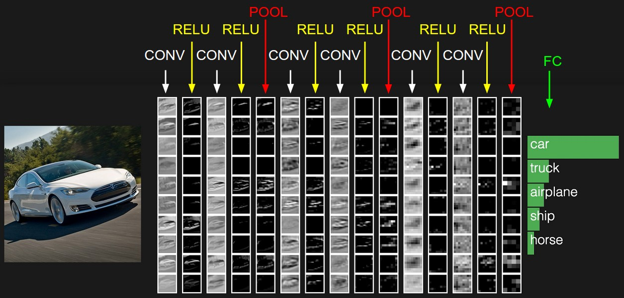
图1 CNN的一般流程

   1.2 CNN中的conv-relu-pool

    首先是conv。也就是卷积，卷积过程与LeNet-5中没有什么差别，具体的细节可能根据实验效果而定。比如对于同样32*32的初始输入，用不同大小窗口采样会得到不同的采样结果（5*5的窗口得到28*28，3*3的窗口得到30*30），窗口大小根据最后准确率来定，所以不太用纠结到底是多大最好。当然可以想见，窗口过大会导致提取的信息过少，窗口过小导致运算量和层与层直接的参数剧增（层与层之间参数个数计算见LeNet-5中的解释）。知道原理即可。

    然后是relu激活函数。猫咪可能听说过神经网络中著名的sigmod函数和tanh函数，relu函数也是激活函数的一种。在这一节就顺便把常用的激活函数函数也给猫咪说啦。本质上，这些激活函数都是做一个映射工作，以sigmod函数为例，它的表达式为，函数图像如图2所示：

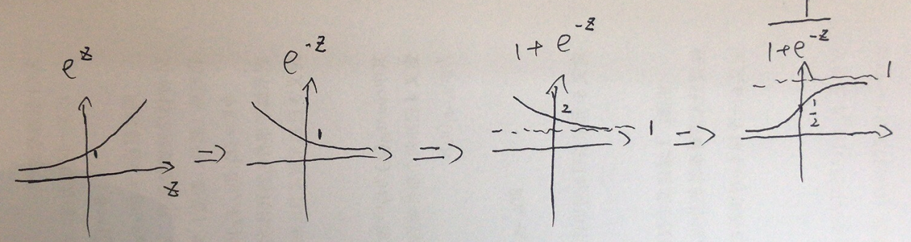图3 sigmod函数图像

参数z可以是一个线性组合（这句话很重要，如图4）。例如conv卷积，使用5*5的窗口后将32*32的初始图片变为28*28后。那么我使用一个步长为4的4*4的窗口（无窗口任何重叠）作为sigmod激活函数的采样窗口，可以得到一个7*7的结果。具体结果的由来如图4所示。也就是说，经过类似sigmod激活函数后，我们进一步的“降采样”并且将矩阵每个元素的值域进行了新的映射（sigmod映射为(0,1)）。

 

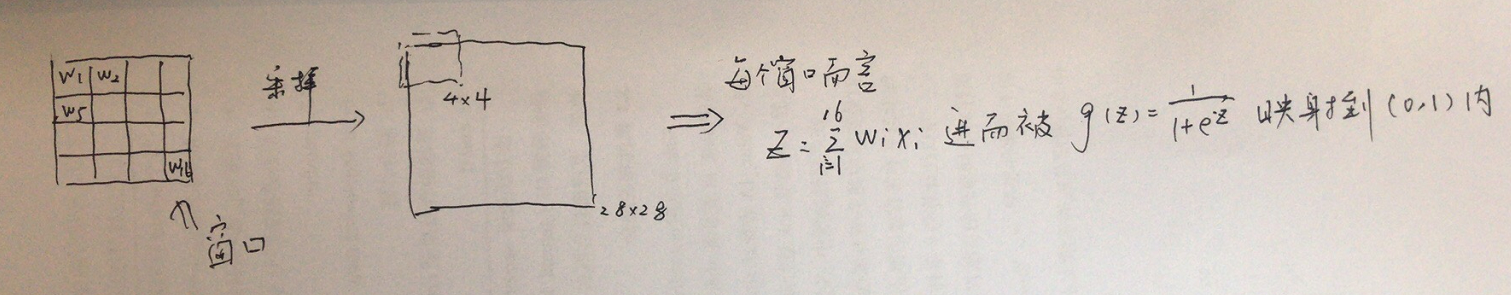
图4 sigmod激活函数工作示例

同样的，relu函数就不再赘述啦（它的表达式比较复杂），只要知道它是通过一个表达式进行映射就可以了。relu的函数图像如下图。可以看到，线性性质会让它更容易收敛，在训练时求导也会更容易（我们不用太关心这个问题，因为都是机器在做嘻嘻，了解就好）。

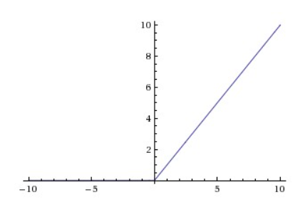图5 relu函数

     接着是pool。在CNN的pool层中使用了maxpool方法。通过LeNet-5的pool层我们知道，这一层主要是为了降采样维度的。maxpool也不例外，它同样也是使用一个采样窗口进行采样，但不再是“加权求和”，而是选用窗口内最大的值最为该区域的代表。例如步长为2，窗口大小2*2的maxpool（无窗口重叠），如图6所示。图中的值只是为了举个例子，如果激活函数使用的sigmod，那么值都应该在（0，1）之间。

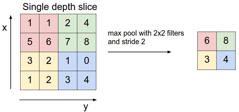图6 maxpool

   1.3 CNN中的全连接层

    和LeNet-5的全连接层没有什么区别。从conv-relu-maxpool层后得到的依然是矩阵。它可能用了类似LeNet-5那样很多的窗口，采样了很多的大小相同的矩阵。到了全连接层就是要综合这些信息。方法和LeNet-5类似。比如从conv-relu-maxpool后得到一个20*20的矩阵，我先设计第一个全连接层输出为20，那么这两层之间的参数个数就为20*20*20+20（如果是y=wx+b形式）。最后再设计一个全连接层，将上一层输出的20映射到第二个全连接层的10个输出（对应数字0-9）即可。

2. 山高天远烟水寒

  2.1 代码

    接下来是代码部分啦。这是一个4层的CNN网络来实现MNIST手写数字识别。这次不需要单独下载数据集（数据集不是很大可以放心食用），数据集写在了import里面更方便猫咪一点。我使用的python3.5和tensorflow1.6.0版本，不用修改可以直接运行。

#---------------------------------------
#
# 简单的4层CNN模型
# 应用于MNIST手写库
#---------------------------------------
#
# 数据集无需单独下载，代码中会下载
# 数据集下载至代码根目录下temp文件中
# temp包含4个.gz文件：测试集的图片和label，训练集的图片和label
#---------------------------------------
#
# Author:ZQH
# Data:2018-04-11
# For cat Dan
#---------------------------------------

import matplotlib.pyplot as plt
import numpy as np
import tensorflow as tf
from tensorflow.contrib.learn.python.learn.datasets.mnist import read_data_sets
from tensorflow.python.framework import ops
ops.reset_default_graph()

# 开始计算图会话
sess = tf.Session()

# 创建temp文件夹，导入数据。数据源自上面import内容
data_dir = 'temp'
mnist = read_data_sets(data_dir)

# 加载数据集，将其reshape为28*28的矩阵
train_xdata = np.array([np.reshape(x, (28,28)) for x in mnist.train.images])
test_xdata = np.array([np.reshape(x, (28,28)) for x in mnist.test.images])

# 转换label为one-hot编码向量（例如1为[0000000001]，8为[010000000]）
train_labels = mnist.train.labels
test_labels = mnist.test.labels

# 设置模型参数。由于图像是灰度图像，图像深度为1，则颜色通道为1
batch_size = 100
learning_rate = 0.005
evaluation_size = 500
image_width = train_xdata[0].shape[0]
image_height = train_xdata[0].shape[1]
target_size = max(train_labels) + 1
num_channels = 1 # 颜色通道=1
generations = 500
eval_every = 5
conv1_features = 25
conv2_features = 50
max_pool_size1 = 2 # N*N窗口大小->第一个max-pool层
max_pool_size2 = 2 # N*N窗口大小->第二个max-pool层
fully_connected_size1 = 100

# 为数据集声明占位符（tensorflow通过占位符获取数据）
# 同时声明训练数据集变量和测试数据集变量
x_input_shape = (batch_size, image_width, image_height, num_channels)
x_input = tf.placeholder(tf.float32, shape=x_input_shape)
y_target = tf.placeholder(tf.int32, shape=(batch_size))
eval_input_shape = (evaluation_size, image_width, image_height, num_channels)
eval_input = tf.placeholder(tf.float32, shape=eval_input_shape)
eval_target = tf.placeholder(tf.int32, shape=(evaluation_size))

# 声明卷积层的权重和偏置
conv1_weight = tf.Variable(tf.truncated_normal([4, 4, num_channels, conv1_features],
                                               stddev=0.1, dtype=tf.float32))
conv1_bias = tf.Variable(tf.zeros([conv1_features], dtype=tf.float32))

conv2_weight = tf.Variable(tf.truncated_normal([4, 4, conv1_features, conv2_features],
                                               stddev=0.1, dtype=tf.float32))
conv2_bias = tf.Variable(tf.zeros([conv2_features], dtype=tf.float32))

# 声明全连接层的权重和偏置
resulting_width = image_width // (max_pool_size1 * max_pool_size2)
resulting_height = image_height // (max_pool_size1 * max_pool_size2)
full1_input_size = resulting_width * resulting_height * conv2_features
full1_weight = tf.Variable(tf.truncated_normal([full1_input_size, fully_connected_size1],
                          stddev=0.1, dtype=tf.float32))
full1_bias = tf.Variable(tf.truncated_normal([fully_connected_size1], stddev=0.1, dtype=tf.float32))
full2_weight = tf.Variable(tf.truncated_normal([fully_connected_size1, target_size],
                                               stddev=0.1, dtype=tf.float32))
full2_bias = tf.Variable(tf.truncated_normal([target_size], stddev=0.1, dtype=tf.float32))


# 声明算法模型。首先创建一个模型函数my_conv_net()
def my_conv_net(input_data):
    # 第一个Conv-ReLU-MaxPool层
    conv1 = tf.nn.conv2d(input_data, conv1_weight, strides=[1, 1, 1, 1], padding='SAME')
    relu1 = tf.nn.relu(tf.nn.bias_add(conv1, conv1_bias))
    max_pool1 = tf.nn.max_pool(relu1, ksize=[1, max_pool_size1, max_pool_size1, 1],
                               strides=[1, max_pool_size1, max_pool_size1, 1], padding='SAME')

    # 第二个Conv-ReLU-MaxPool层
    conv2 = tf.nn.conv2d(max_pool1, conv2_weight, strides=[1, 1, 1, 1], padding='SAME')
    relu2 = tf.nn.relu(tf.nn.bias_add(conv2, conv2_bias))
    max_pool2 = tf.nn.max_pool(relu2, ksize=[1, max_pool_size2, max_pool_size2, 1],
                               strides=[1, max_pool_size2, max_pool_size2, 1], padding='SAME')

    # 把输出“铺平”为1*N的向量，为全连接层的计算做准备
    final_conv_shape = max_pool2.get_shape().as_list()
    final_shape = final_conv_shape[1] * final_conv_shape[2] * final_conv_shape[3]
    flat_output = tf.reshape(max_pool2, [final_conv_shape[0], final_shape])

    # 第一个全连接层
    fully_connected1 = tf.nn.relu(tf.add(tf.matmul(flat_output, full1_weight), full1_bias))

    # 第二个全连接层
    final_model_output = tf.add(tf.matmul(fully_connected1, full2_weight), full2_bias)
   
    return(final_model_output)

# 声明训练模型
model_output = my_conv_net(x_input)
test_model_output = my_conv_net(eval_input)

# 因为预测结果是单分类（0-9哪个数字），所以使用softmax函数为损失函数
loss = tf.reduce_mean(tf.nn.sparse_softmax_cross_entropy_with_logits(logits=model_output, labels=y_target))

# 创建训练集、测试集和预测函数
prediction = tf.nn.softmax(model_output)
test_prediction = tf.nn.softmax(test_model_output)

# 创建精度函数，评估模型准确度
def get_accuracy(logits, targets):
    batch_predictions = np.argmax(logits, axis=1)
    num_correct = np.sum(np.equal(batch_predictions, targets))
    return(100. * num_correct/batch_predictions.shape[0])

# 创建优化器函数，声明训练步长
my_optimizer = tf.train.MomentumOptimizer(learning_rate, 0.9)
train_step = my_optimizer.minimize(loss)

# 初始化模型变量
init = tf.global_variables_initializer()
sess.run(init)

# 开始训练。迭代500次后可以达到96%~97%准确度
# 没有LeNet高是因为网络层数不够深等原因
train_loss = []
train_acc = []
test_acc = []
for i in range(generations):
    rand_index = np.random.choice(len(train_xdata), size=batch_size)
    rand_x = train_xdata[rand_index]
    rand_x = np.expand_dims(rand_x, 3)
    rand_y = train_labels[rand_index]
    train_dict = {x_input: rand_x, y_target: rand_y}
   
    sess.run(train_step, feed_dict=train_dict)
    temp_train_loss, temp_train_preds = sess.run([loss, prediction], feed_dict=train_dict)
    temp_train_acc = get_accuracy(temp_train_preds, rand_y)
   
    if (i+1) % eval_every == 0:
        eval_index = np.random.choice(len(test_xdata), size=evaluation_size)
        eval_x = test_xdata[eval_index]
        eval_x = np.expand_dims(eval_x, 3)
        eval_y = test_labels[eval_index]
        test_dict = {eval_input: eval_x, eval_target: eval_y}
        test_preds = sess.run(test_prediction, feed_dict=test_dict)
        temp_test_acc = get_accuracy(test_preds, eval_y)
       
        # 记录并输出结果
        train_loss.append(temp_train_loss)
        train_acc.append(temp_train_acc)
        test_acc.append(temp_test_acc)
        acc_and_loss = [(i+1), temp_train_loss, temp_train_acc, temp_test_acc]
        acc_and_loss = [np.round(x,2) for x in acc_and_loss]
        print('Generation # {}. Train Loss: {:.2f}. Train Acc (Test Acc): {:.2f} ({:.2f})'.format(*acc_and_loss))
   
   
# 使用Matplotlib模块绘制损失函数和准确度函数
eval_indices = range(0, generations, eval_every)
# 损失函数
plt.plot(eval_indices, train_loss, 'k-')
plt.title('Softmax Loss per Generation')
plt.xlabel('Generation')
plt.ylabel('Softmax Loss')
plt.show()

# 训练和测试时的准确度函数
plt.plot(eval_indices, train_acc, 'k-', label='Train Set Accuracy')
plt.plot(eval_indices, test_acc, 'r--', label='Test Set Accuracy')
plt.title('Train and Test Accuracy')
plt.xlabel('Generation')
plt.ylabel('Accuracy')
plt.legend(loc='lower right')
plt.show()

2.2 运行结果

训练共计500轮。输出除了训练的准确度外，还将loss和准确度信息记录下来绘制图形更直观一点。如下图所示。

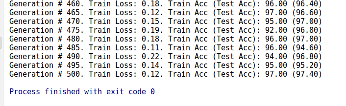
图X 500轮后训练结果

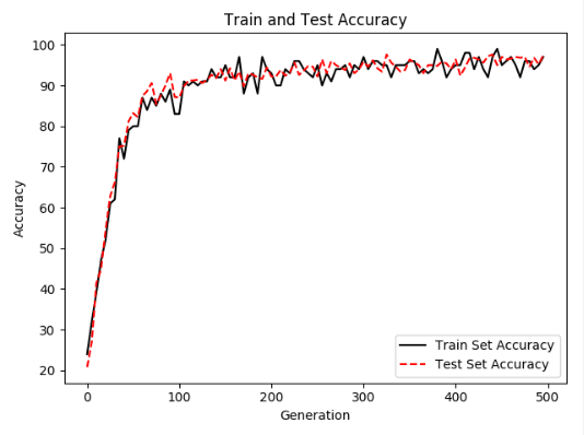
图X 训练和测试时的准确率

图X softmax作为损失函数的变化情况

3. 相思枫叶丹

  本文就先到这里啦。其实回头来看的话，CNN在LeNet-5的基础上最大的进步就是在conv-relu-pool这里，它采用了更多的非线性因素，而不像LeNet-5重复进行采样和降维。可能更多的细节和参数

需要猫咪去代码里面体会，但大概的过程确实如此。我们在学习神经网络和机器学习过程中，要学会应用（不求甚解），但熟练了就会发现好像也就那么回事。因为最难的计算部分是计算机做的，最有

创造性的算法是别人写的嘻嘻~

代码是一定调通了哒，注释也检查了很多遍了。希望能对猫咪有帮助。有疑问可以和秋涵君一起讨论~

一重山，两重山，山高天远烟水寒，相思枫叶丹。今天，也是爱喵的一天。