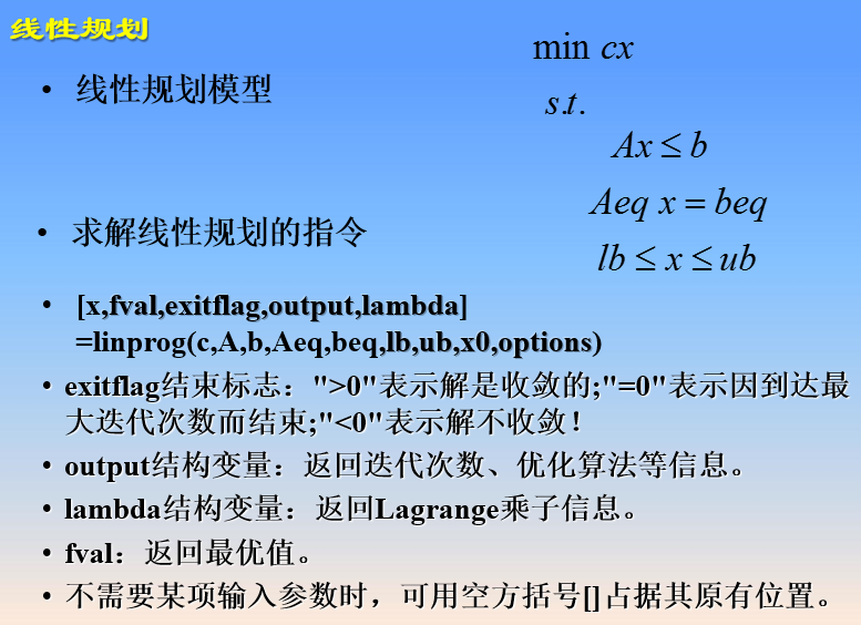
Minf(x)=-5x1 -4x2 -6x3
x1 -x2 +x3 <=20
3x1 +2x2 +4x3 <=42
3x1 +2x2 <=30
0<=x1,0<=x2,0<=x3
>> c=[-5,-4,-6];
>> A=[1 -1 1
3 2 4
3 2 0];
>> b=[20;42;30];
>> lb=zeros(3,1);
>> [x,fval,exitflag,output,lambda]=linprog(c,A,b,[],[],lb)
Optimization terminated.

x =

    0.0000
   15.0000
    3.0000


fval =

  -78.0000


exitflag =

     1


output =

         iterations: 6
          algorithm: 'interior-point-legacy'
       cgiterations: 0
            message: 'Optimization terminated.'
    constrviolation: 0
      firstorderopt: 5.8705e-10


lambda =

    ineqlin: [3x1 double]
      eqlin: [0x1 double]
      upper: [3x1 double]
      lower: [3x1 double]

>>
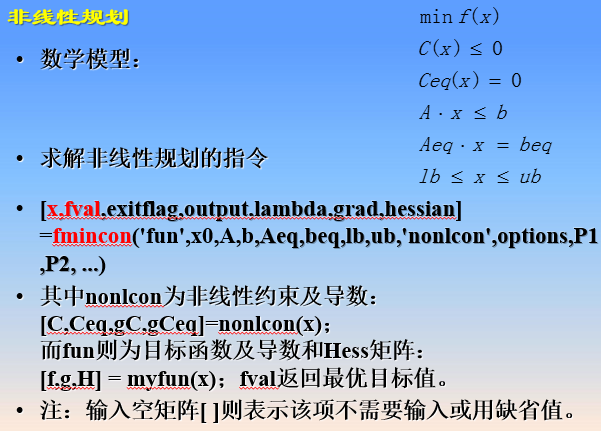

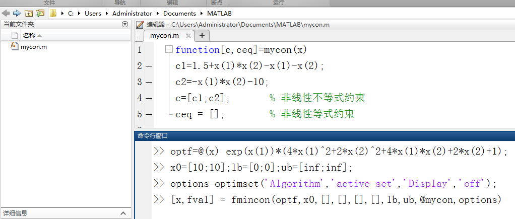
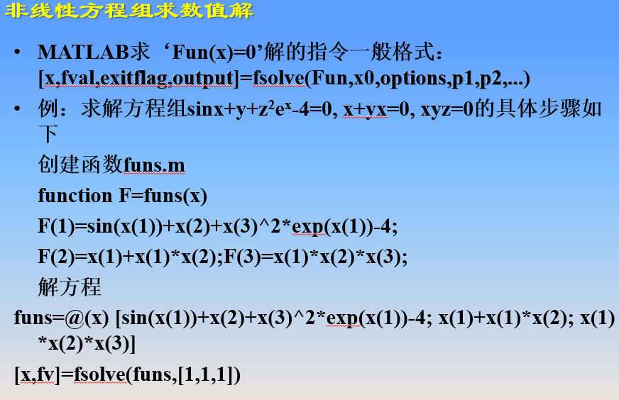
function[c,ceq]=mycon(x)
c1=1.5+x(1)*x(2)-x(1)-x(2);
c2=-x(1)*x(2)-10;
c=[c1;c2];       % 非线性不等式约束
ceq = [];        % 非线性等式约束
>> optf=@(x) exp(x(1))*(4*x(1)^2+2*x(2)^2+4*x(1)*x(2)+2*x(2)+1);
>> x0=[10;10];lb=[0;0];ub=[inf;inf];
>> options=optimset('Algorithm','active-set','Display','off');
>> [x,fval] = fmincon(optf,x0,[],[],[],[],lb,ub,@mycon,options)

x =

         0
    1.5000


fval =

    8.5000

>>

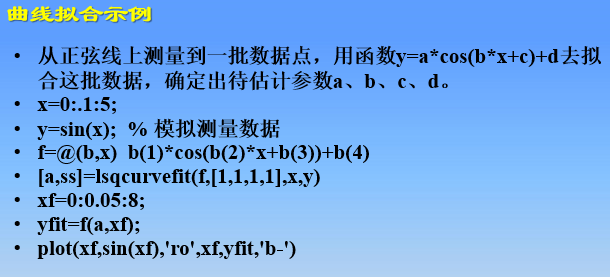
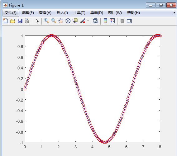
>> x=0:.1:5;
>> y=sin(x);
>> f=@(b,x)  b(1)*cos(b(2)*x+b(3))+b(4);
>> [a,ss]=lsqcurvefit(f,[1,1,1,1],x,y)

Local minimum found.

Optimization completed because the size of the gradient is less than
the default value of the function tolerance.

<stopping criteria details>


a =

   -1.0000    1.0000    1.5708   -0.0000


ss =

   8.7594e-29

>> xf=0:0.05:8;
yfit=f(a,xf);
plot(xf,sin(xf),'ro',xf,yfit,'b-')
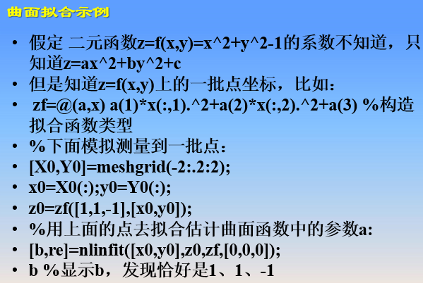
>> zf=@(a,x) a(1)*x(:,1).^2+a(2)*x(:,2).^2+a(3) %构造拟合函数类型

zf =

    @(a,x)a(1)*x(:,1).^2+a(2)*x(:,2).^2+a(3)

>> [X0,Y0]=meshgrid(-2:.2:2);
x0=X0(:);y0=Y0(:);
z0=zf([1,1,-1],[x0,y0]);
>> %用上面的点去拟合估计曲面函数中的参数a:
>> [b,re]=nlinfit([x0,y0],z0,zf,[0,0,0]);
b %显示b,发现恰好是1、1、-1

b =

    1.0000    1.0000   -1.0000

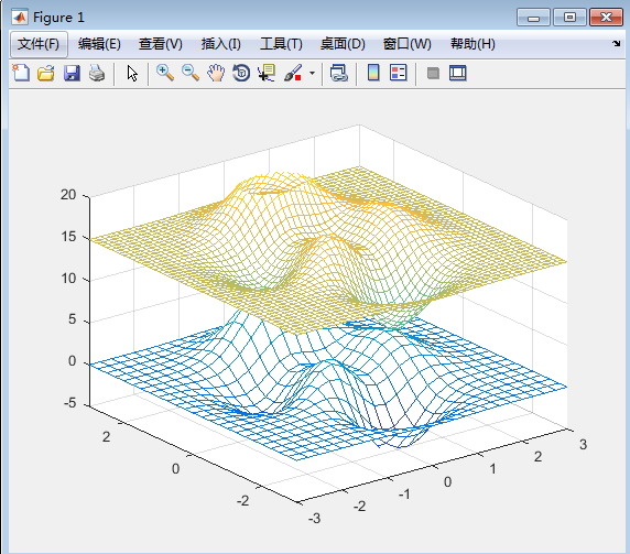
>> [X,Y] = meshgrid(-3:.25:3);Z = peaks(X,Y);
[XI,YI] = meshgrid(-3:.125:3);
ZI = interp2(X,Y,Z,XI,YI);
mesh(X,Y,Z), hold, mesh(XI,YI,ZI+15), hold off
axis([-3 3 -3 3 -5 20])
已锁定最新绘图
>>