数据分析之NumPy，pandas，Matplotlib

安装Anaconda

Anaconda在官网就可以下载，网址：https://www.anaconda.com/download/  ，官网上可以选择各个操作系统的安装包。

双击下载下来的.exe文件就可以安装了

安装时将两个选项都选上，将安装路径写入环境变量，然后等待安装完成就可以了。

安装完成后，打开Windows的命令行窗口：按Win+R键打开窗口，输入cmd。打开Windows的命令提示符输入conda list 就可以查询现在安装了哪些库，常用的numpy, scipy等安装上就可以啦~

        —     输入 conda --version 验证并查看版本

        —     输入 conda list 命令可以看已经安装的python包

        —     输入 jupyter notebook, 直接浏览器打开，可以在上面写，执行

如果你还有什么包没有安装上，可以运行conda install ***  来进行安装（***为需要的包的名称）。如果某个包版本不是最新的，运行 conda update *** 就可以更新了

• anaconda
  • 官网：https://www.anaconda.com/
  • 集成环境：集成好了数据分析和机器学习中所需要的全部环境
    • 注意：
      • 安装目录不可以有中文和特殊符号
• jupyter
  • jupyter就是anaconda提供的一个基于浏览器的可视化开发工具
• jupyter的基本使用
  • 启动：在终端中录入：jupyter notebook的指令，按下回车
  • 新建：
    • python3：anaconda中的一个源文件
    • cell有两种模式：
      • code：编写代码
      • markdown：编写笔记
  • 快捷键：
    • 添加cell：a或者b
    • 删除：x
    • 修改cell的模式：
      • m：修改成markdown模式
      • y：修改成code模式
    • 执行cell：
      • shift+enter
    • tab：自动补全
    • 代开帮助文档：shift+tab

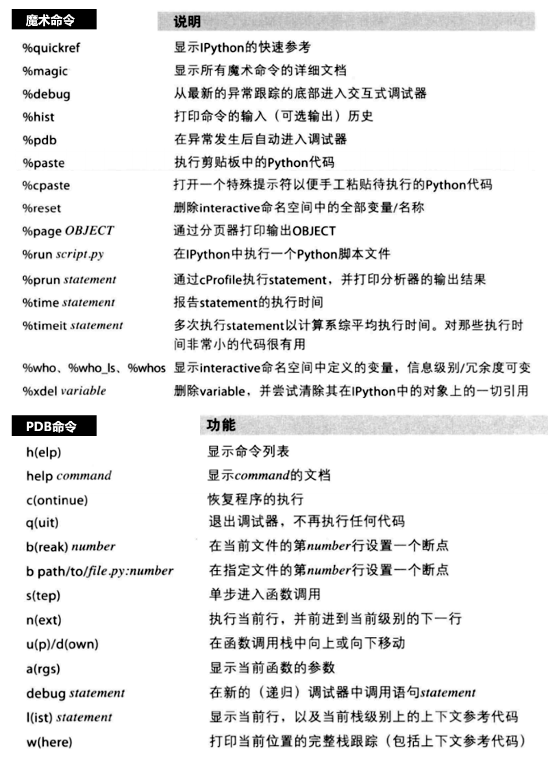
IPython

 

 

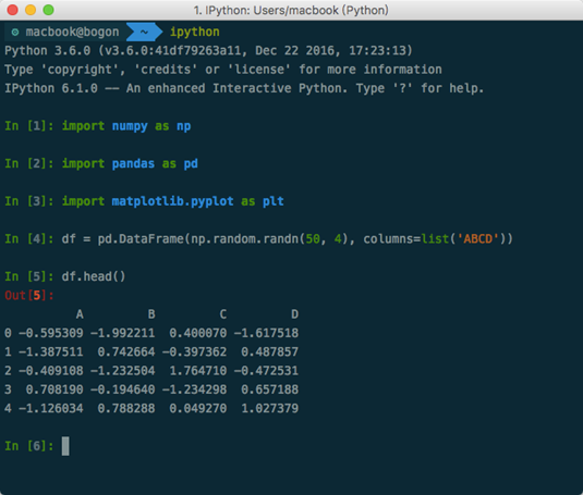
• IPython:交互式的Python命令行
• 安装:pip3 install ipython
• 使用:ipython
• 快捷键：
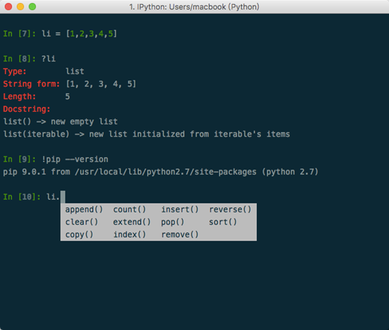
  1. TAB键自动完成
  2. ?：内省、命名空间搜索      a?      a.append?     a.*pp*?
  3. !：执行系统命令    !cd
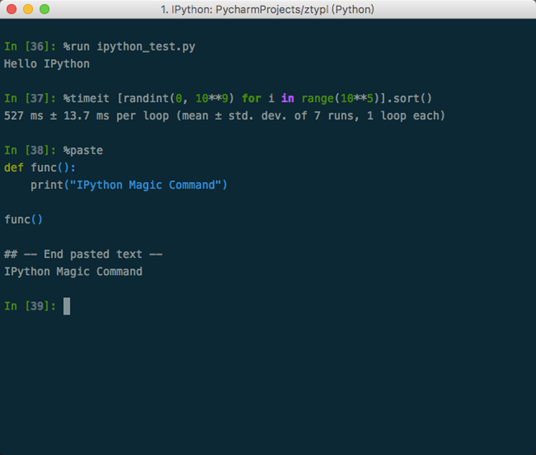
• 魔术命令：以%开始的命令
  1. %run：执行文件代码
  2. %paste：执行剪贴板代码
  3. %timeit：评估运行时间    %timeit a.sort()
  4. %pdb：自动调试 %pdb on      n      %pdb off
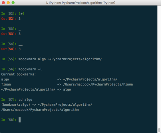
• 使用命令历史    _
• 获取输入输出结果
• 目录标签系统
• IPython Notebook

NumPy模块

NumPy是高性能科学计算和数据分析的基础包。它是pandas等其他各种工具的基础。

• 安装方法：pip3 install numpy
• 引用方式：import numpy as np
• NumPy的主要功能：
  1. ndarray，一个多维数组结构，高效且节省空间
  2. 无需循环对整组数据进行快速运算的数学函数
  3. 读写磁盘数据的工具以及用于操作内存映射文件的工具
  4. 线性代数、随机数生成和傅里叶变换功能
  5. 用于集成C、C++等代码的工具

一、ndarray多维数组对象

• 创建ndarray：np.array(array_like)
• ndarray是多维数组结构，与列表的区别是：
  1. 数组对象内的元素类型必须相同
  2. 数组大小不可修改

1、ndarray常用属性

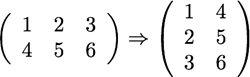
• T 数组的转置（对高维数组而言）
• dtype 数组元素的数据类型
• size 数组元素的个数
• ndim 数组的维数
• shape 数组的维度大小（以元组形式）

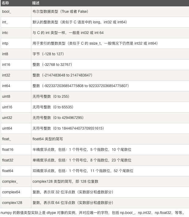
2、ndarray数据类型

• 布尔型：bool_
• 整型：int_ int8 int16 int32 int64
• 无符号整型：uint8 uint16 uint32 uint64
• 浮点型：float_ float16 float32 float64
• 复数型：complex_ complex64 complex128

3、ndarray创建

• array() 将列表转换为数组，可选择显式指定dtype
• arange() range的numpy版，支持浮点数
• linspace() 类似arange()，第三个参数为数组长度
• zeros() 根据指定形状和dtype创建全0数组
• ones() 根据指定形状和dtype创建全1数组
• empty() 根据指定形状和dtype创建空数组（随机值）
• eye() 根据指定边长和dtype创建单位矩阵

4、ndarray索引和切片

• 数组和标量之间的运算：
  1. a+1     a*3     1//a     a**0.5     a>5
• 同样大小数组之间的运算：
  1. a+b     a/b     a**b     a%b       a==b
• 数组的索引：
  1. 一维数组：a[5]
  2. 多维数组：
     1. 列表式写法：a[2][3]
     2. 新式写法：a[2,3] (推荐)
• 数组的切片：
  1. 一维数组：a[5:8]     a[4:]     a[2:10] = 1
  2. 多维数组：a[1:2, 3:4]     a[:,3:5]     a[:,1]
  3. 与列表不同，数组切片时并不会自动复制，在切片数组上的修改会影响原数组。 【解决方法：copy()】
  4. copy()方法开源创建数组的深拷贝

5、布尔型索引

问题：给一个数组，选出数组中所有大于5的数。
答案：a[a>5]
原理：
a>5会对a中的每一个元素进行判断，返回一个布尔数组
布尔型索引：将同样大小的布尔数组传进索引，会返回一个由所有True对应位置的元素的数组

问题2：给一个数组，选出数组中所有大于5的偶数。
问题3：给一个数组，选出数组中所有大于5的数和偶数。
答案：
a[(a>5) & (a%2==0)]
a[(a>5) | (a%2==0)

6、花式索引*

问题1：对于一个数组，选出其第1，3，4，6，7个元素，组成新的二维数组。
答案：a[[1,3,4,6,7]]

问题2：对一个二维数组，选出其第一列和第三列，组成新的二维数组。
答案：a[:,[1,3]]

二、NumPy：通用函数

ceil:向上取整 3.6 -》4 3.1-》4 -3.1-》-3

floor:向下取整：3.6-》3 3.1-》3 -3.1-》-4

round:四舍五入：3.6-》4 3.1-》3 -3.6-》-4

trunc(int):向零取整（舍去小数点后） 3.6-》3 3.1-》3 -3.1-》-3

arr = np.arange(10)
arr.sum()#45  求和
arr.mean()#4.5 平均值
arr.cumsum()  #array([ 0,  1,  3,  6, 10, 15, 21, 28, 36, 45], dtype=int32) #等差数列 
arr.std() #、求标准差

通用函数：能同时对数组中所有元素进行运算的函数
常见通用函数：
一元函数：abs(绝对值), sqrt(开方), exp, log, ceil, floor, rint, trunc, modf(分别取出小数部分和整数部分), isnan, isinf, cos, sin, tan
二元函数：add, substract, multiply, divide, power, mod, maximum, mininum,

三、补充知识：浮点数特殊值

浮点数：float
浮点数有两个特殊值：
nan(Not a Number)：不等于任何浮点数（nan != nan）
inf(infinity)：比任何浮点数都大

NumPy中创建特殊值：np.nan    np.inf
在数据分析中，nan常被用作表示数据缺失值

四、数学和统计方法

sum    求和
cumsum 求前缀和
mean    求平均数
std    求标准差
var    求方差
min    求最小值
max    求最大值
argmin    求最小值索引
argmax    求最大值索引

五、随机数生成

随机数生成函数在np.random子包内
常用函数
rand        给定形状产生随机数组（0到1之间的数）
randint        给定形状产生随机整数
choice        给定形状产生随机选择
shuffle        与random.shuffle相同
uniform        给定形状产生随机数组

import numpy as np
import random
a=[random.uniform(10.0,20.0) for i in range(3)]
print(a)
a=np.array(a)  #将列表转换成数组
print(a)
x=10
print(a*x) #数组里面的每一项乘以10
print(a.size,a.dtype)#size 数组元素的个数 #dtype 数组元素的数据类型


b=np.array([[1,2],[11,22],[99,99]])
print(b.shape) #shape 数组的维度大小（以元组形式）
print(b.T) #T 数组的转置（对高维数组而言）


c=np.array([[[1,2,3],[666,777,888]],[[11,22,33],[55,66,77]]])
print(c.shape)
print(c.ndim) #ndim 数组的维数


d=np.zeros(10)
print(d)
d=np.zeros(10,dtype='int') #可以加dtype指定类型，默认是float
print(d)
d=np.ones(10)
print(d)


d=np.empty(10)  ##注意内存残留
print(d)
d=np.arange(2,10,3)
print(d)
d=np.arange(2,10,0.3) ##步长可以是小数
print(d)

d=np.linspace(1,10,3) ##最后一个参数是分成多少份数,也就是数组长度，步长是一样的
print(d)

d=np.eye(10)
print(d)

a=np.arange(10)
print(a,a+1,a*3) #每一列加1，每一列乘以3
b=np.arange(10,20)
print(b,a+b) #对应列相加，前提是数组长度一样
a[0]=100
print(a>b) #每一列的比较返回布尔，整体返回布尔列表

a=np.arange(15)
print(a)
a=np.arange(15).reshape((3,5))  #生成一个3行5列的二维数组
print(a,a.shape)
print(a[0][0],a[0,0]) # 推荐a[0,0]的写法


a=np.arange(15)
b=np.arange(10)
c=a[0:4]
d=b[0:4].copy() #这样就不影响b,这个是复制出来了一份
c[0]=20  #对c进行修改同样会影响到a,是出于省空间的考量，其实只是把地址指向了a的前4项
d[0]=20
print(a,b,c,d)


a=np.arange(15).reshape((3,5))
print(a[0][0:2],a[1,0:2])
print(a[0:2]) #默认是按行切
print(a[0:2,0:2]) #逗号前面是行，后面是列，得到的还是二维数组

print(a[1:4,2:4])
print(a[1:,2:4])


a=[random.randint(0,10) for i in range(20)]
print(list(filter(lambda x:x>5,a)))
a=np.array(a)
print(a>5) #[False False ... True  True]
print(a[a>5])  #a>5会把列表的每一项先转换成True和False

#方式1：
b=a[a>5]
print(b[b%2==0],'所有大于5的偶数')
#方式2：
print(a[(a>5) & (a%2==0)])#记得加括号，&的优先级比较高

print(3 and 4,3 & 4)
print(a[(a>5) | (a%2==0)])#大于5或者偶数

a=np.arange(4)
print(a)
print(a[[True,True,False,False]]) #是True的才显示


a=np.arange(10,20)
print(a)
print(a[[1,3,4]],'花式索引') #

a=np.arange(20).reshape(4,5)
print(a[0,2:4])
print(a[0,a[0]>2])

print(a[[1,3],[1,3]])# 注意：这个是取出（1,1）和（3,3）位置上的数，
print(a[[1,3],:][:,[1,3]]) # 花式索引要这样操作

a=np.arange(-5,5)
print(np.abs(a))
print(abs(a))
# print(np.sqrt(a))

import math
a=1.6
print(math.trunc(a),math.ceil(a),round(a),math.floor(a))
print(np.trunc(a),np.ceil(a),np.round(a),np.floor(a))

print(np.modf(a))#把整数和小数部位分开，返回一个元组，元组第一个值是小数部分，第二个值是整数部分

#nan(Not a Number)：不等于任何浮点数（nan != nan）
#inf(infinity)：比任何浮点数都大
print(float('nan'),float('inf')) #nan inf
print(np.nan == np.nan) #False
print(np.isnan(np.nan)) #True
print(~ np.isnan(np.nan)) #False
print(not np.isnan(np.nan)) #False

print(np.inf == np.inf) #True


a=np.arange(0,5)
b=5/a #inf
c=a/a #nan
print(b,)
print(c[~np.isnan(c)])  #去掉nan
print(b[~np.isinf(b)])  #去掉inf


a=np.array([3,4,5,6,7])
b=np.array([2,5,3,7,4])
print(np.maximum(a,b))
print(a.sum())
print(a.mean())

"""
方差是在概率论和统计方差衡量随机变量或一组数据时离散程度的度量。
1,2,3,4,5
方差: ((1-3)**2+(2-3)**2+(3-3)**2+(4-3)**2+(5-3)**2)/5
标准差：方差再开方 
sqrt(((1-3)**2+(2-3)**2+(3-3)**2+(4-3)**2+(5-3)**2)/5)
"""



a=np.arange(0,10,0.2)
print(a.var(),a.std()) #方差 标准差
print(a.mean()-a.std(),a.mean()+a.std())
print(a.mean()-2*a.std(),a.mean()+2*a.std())

print(a.argmax()) #取最大数的索引

a=np.random.randint(0,10,10) #第三个参数是数组长度
a=np.random.randint(0,10,(3,5)) #第三个参数三行五列
a=np.random.randint(0,10,(3,5,4)) #第三个参数三行五列
a=np.random.rand(10) #####代表个数  不是random.random
print(a)

# x=np.linspace(-10,10,10000)
# y=x**2
# import matplotlib.pyplot as plt
# plt.plot(x,y)
# plt.show()

pandas

pandas是一个强大的Python数据分析的工具包，pandas是基于NumPy构建的。

• 安装方法：pip3 install pandas
• 引用方式：import pandas as pd
• pandas的主要功能：
  1. 具备对其功能的数据结构DataFrame、Series
  2. 集成时间序列功能
  3. 提供丰富的数学运算和操作
  4. 灵活处理缺失数据

一、Series

Series（数组+字典）是一种类似于一位数组的对象，由一组数据和一组与之相关的数据标签（索引）组成。

1、创建方式

pd.Series([4,7,-5,3]) 
pd.Series([4,7,-5,3],index=['a','b','c','d'])               
pd.Series({'a':1, 'b':2})             
pd.Series(0, index=['a','b','c','d’])

2、Series特性

Series支持数组的特性：
从ndarray创建Series：Series(arr)
与标量运算：sr*2
两个Series运算：sr1+sr2
索引：sr[0], sr[[1,2,4]]
切片：sr[0:2]（切片依然是视图形式）
通用函数：np.abs(sr)
布尔值过滤：sr[sr>0]
统计函数：mean() sum() cumsum()

Series支持字典的特性（标签）：
从字典创建Series：Series(dic), 
in运算：’a’ in sr、for x in sr
键索引：sr['a'], sr[['a', 'b', 'd']]
键切片：sr['a':'c']
其他函数：get('a', default=0)等

3、Series整数索引

整数索引的pandas对象往往会使新手抓狂。
例：
sr = np.Series(np.arange(4.))
sr[-1] 

如果索引是整数类型，则根据整数进行数据操作时总是面向标签的。
loc属性        以标签解释
iloc属性        以下标解释 

4、Series数据对齐

pandas在运算时，会按索引进行对齐然后计算。如果存在不同的索引，则结果的索引是两个操作数索引的并集。

例：
sr1 = pd.Series([12,23,34], index=['c','a','d'])
sr2 = pd.Series([11,20,10], index=['d','c','a',])
sr1+sr2
sr3 = pd.Series([11,20,10,14], index=['d','c','a','b'])
sr1+sr3

如何在两个Series对象相加时将缺失值设为0？
sr1.add(sr2, fill_value=0)
灵活的算术方法：add, sub, div, mul

5、Series缺失数据

缺失数据：使用NaN（Not a Number）来表示缺失数据。其值等于np.nan。内置的None值也会被当做NaN处理。
处理缺失数据的相关方法：
dropna()        过滤掉值为NaN的行
fillna()        填充缺失数据
isnull()        返回布尔数组，缺失值对应为True
notnull()        返回布尔数组，缺失值对应为False

过滤缺失数据：sr.dropna() 或 sr[data.notnull()]
填充缺失数据：fillna(0)

二、DataFrame

1、创建方式

DataFrame是二维数据对象
DataFrame是一个表格型的数据结构，含有一组有序的列。
DataFrame可以被看做是由Series组成的字典，并且共用一个索引。

创建方式：
pd.DataFrame({'one':[1,2,3,4],'two':[4,3,2,1]})
pd.DataFrame({'one':pd.Series([1,2,3],index=['a','b','c']), 'two':pd.Series([1,2,3,4],index=['b','a','c','d'])})
......

csv文件读取与写入：
df.read_csv('filename.csv')
df.to_csv()

2、DataFrame常用属性及方法

index                    获取索引
T                        转置
columns                    获取列索引
values                    获取值数组
describe()                获取快速统计

DataFrame各列name属性：列名
rename(columns={})

3、DataFrame索引和切片

DataFrame是一个二维数据类型所以有行索引和列索引。

DataFrame同样可以通过标签和位置两种方法进行索引和切片。

loc属性和iloc属性
使用方法：逗号隔开，前面是行索引，后面是列索引
行/列索引部分可以是常规索引、切片、布尔值索引、花式索引任意搭配。

DataFrame使用索引切片：

方法1：两个中括号，先取列再取行。    df['A'][0]
方法2（推荐）：使用loc/iloc属性，一个中括号，逗号隔开，先取行再取列。
loc属性：解释为标签
iloc属性：解释为下标
向DataFrame对象中写入值时只使用方法2
行/列索引部分可以是常规索引、切片、布尔值索引、花式索引任意搭配。（注意：两部分都是花式索引时结果可能与预料的不同）

通过标签获取：
df['A']
df[['A', 'B']]
df['A'][0]
df[0:10][['A', 'C']]
df.loc[:,['A','B']]
df.loc[:,'A':'C']
df.loc[0,'A']
df.loc[0:10,['A','C']]

通过位置获取：
df.iloc[3]
df.iloc[3,3]
df.iloc[0:3,4:6]
df.iloc[1:5,:]
df.iloc[[1,2,4],[0,3]]

通过布尔值过滤：
df[df['A']>0]
df[df['A'].isin([1,3,5])]
df[df<0] = 0

4、DataFrame数据对齐与缺失数据

DataFrame对象在运算时，同样会进行数据对齐，行索引与列索引分别对齐。
结果的行索引与列索引分别为两个操作数的行索引与列索引的并集。

DataFrame处理缺失数据的相关方法：
dropna(axis=0,where='any',…)
fillna()
isnull()
notnull()

三、pandas其他常用方法

pandas常用方法（适用Series和DataFrame）：
mean(axis=0,skipna=False)
sum(axis=1)
sort_index(axis, …, ascending)        按行或列索引排序
sort_values(by, axis, ascending)    按值排序
NumPy的通用函数同样适用于pandas

apply(func, axis=0)    将自定义函数应用在各行或者各列上                                  ，func可返回标量或者Series
applymap(func)        将函数应用在DataFrame各个元素上
map(func)        将函数应用在Series各个元素上

四、pandas时间对象处理

时间序列类型：
时间戳：特定时刻
固定时期：如2017年7月
时间间隔：起始时间-结束时间
Python标准库：datetime
date time datetime timedelta
dt.strftime()
strptime()
灵活处理时间对象：dateutil包
dateutil.parser.parse()
成组处理时间对象：pandas
pd.to_datetime(['2001-01-01', '2002-02-02'])

产生时间对象数组：date_range
start        开始时间
end        结束时间
periods        时间长度
freq        时间频率，默认为'D'，可选H(our),W(eek),B(usiness),S(emi-)M(onth),(min)T(es), S(econd), A(year),…

五、pandas时间序列

时间序列就是以时间对象为索引的Series或DataFrame。

datetime对象作为索引时是存储在DatetimeIndex对象中的。

时间序列特殊功能：
传入“年”或“年月”作为切片方式
传入日期范围作为切片方式
丰富的函数支持：resample(), strftime(), ……
批量转换为datetime对象：to_pydatetime()

六、pandas从文件读取

读取文件：从文件名、URL、文件对象中加载数据
read_csv        默认分隔符为csv
read_table    默认分隔符为\t
read_excel    读取excel文件  pip3 install xlrd
读取文件函数主要参数：
sep        指定分隔符，可用正则表达式如'\s+'
header=None    指定文件无列名
name        指定列名
index_col    指定某列作为索引
skip_row        指定跳过某些行
na_values    指定某些字符串表示缺失值
parse_dates    指定某些列是否被解析为日期，布尔值或列表

七、pandas写入到文件

写入到文件：
to_csv
写入文件函数的主要参数：
sep
na_rep        指定缺失值转换的字符串，默认为空字符串
header=False    不输出列名一行
index=False    不输出行索引一列
cols        指定输出的列，传入列表

其他文件类型：json, XML, HTML, 数据库
pandas转换为二进制文件格式（pickle）:
save
load

import pandas as pd
import numpy as np
print(pd.Series([2,3,4,5]))
print(pd.Series(np.arange(5)))

sr=pd.Series({'a':1,'b':2})
print(sr)

sr = pd.Series([2,3,4,5],index=['a','b','c','d'])
print(sr,sr[0],sr['a'])
"""
a    2
b    3
c    4
d    5
dtype: int64 2 2
"""

print(sr * 2)
print(sr+sr) # 每列相加

print(sr[0:2])
print(sr['a':'c']) #标签进行切片
print(sr[[1,2]]) #花式索引
print(sr[sr > 2]) #布尔索引
print(sr[['a','b']]) #键索引
print('a' in sr) #True

for i in sr:
    print(i)  #是值不是索引

print(sr.index,sr.values)

######################################整数索引
sr=pd.Series(np.arange(20))
sr2=sr[10:].copy()
print(sr2,sr2[10])  ##10规定解释为标签，不是索引
# print(sr2[-1]) #### 报错
print(sr2.loc[10]) ## 标签
print(sr2.iloc[-1])## 下标

sr1=pd.Series([1,2,3],index=['c','b','a'])
sr2=pd.Series([10,20,30],index=['a','b','c'])
print(sr1+sr2) ##按照标签进行计算

sr1=pd.Series([1,2,3],index=['c','b','a'])
sr2=pd.Series([10,20,30,40],index=['a','b','c','d'])
print(sr1+sr2)

sr1=pd.Series([1,2,3],index=['c','d','a'])
sr2=pd.Series([10,20,30],index=['a','b','c'])
print(sr1.add(sr2,fill_value=0))
sr=sr1+sr2
print(sr.isnull()) ######不是isnan
print(sr.notnull())
print(sr[sr.notnull()])
print(sr.dropna()) ###去掉NaN

print(sr.fillna(0))
print(sr.fillna(sr.mean()))

################################
df = pd.DataFrame({'one':[1,2,3],'two':[4,5,6]})
print(df)
df = pd.DataFrame({'one':[1,2,3],'two':[4,5,6]},index=['a','b','c'])
print(df)
"""
   one  two
0    1    4
1    2    5
2    3    6

   one  two
a    1    4
b    2    5
c    3    6
"""

df = pd.DataFrame({'one':pd.Series([1,2,3],index=['a','b','c']),
                   'two':pd.Series([1,2,3,4],index=['b','a','c','d'])})
print(df)
"""
   one  two
a  1.0    2
b  2.0    1
c  3.0    3
d  NaN    4
"""

print('####################################')
#NaN不参与排序，统一放最后面
print(df.sort_values(by='two')) #按列排序
"""
   one  two
b  2.0    1
a  1.0    2
c  3.0    3
d  NaN    4
"""
print(df.sort_values(by='two',ascending=False)) #按列倒序
print(df.sort_values(by='a',axis=1)) #按行排序，一般不用


print(df.sort_index(),'按索引排序') #按索引排序
"""
   one  two
a  1.0    2
b  2.0    1
c  3.0    3
d  NaN    4 按索引排序
"""
print(df.sort_index(ascending=False))
print(df.sort_index(ascending=False,axis=1))



print(df['one']['a'],'先是列后是行')  #########注意
print(df.loc['a','one']) #########推荐先行后列

print(df.loc['a',:])
print(df.loc['a',])
#行/列索引部分可以是常规索引、切片、布尔值索引、花式索引任意搭配。
print(df.loc[['a','c'],:])
print(df.loc[['a','c'],'two'])

print(df.mean()) #每一列的平均值
print(df.mean(axis=1),'每一行的平均值') #每一行的平均值
"""
one    2.0
two    2.5
dtype: float64

a    1.5
b    1.5
c    3.0
d    4.0
dtype: float64 每一行的平均值
"""
print(df.sum())
print(df.sum(axis=1))
"""
one     6.0
two    10.0
dtype: float64

a    3.0
b    3.0
c    6.0
d    4.0
dtype: float64
"""


df2=pd.DataFrame({'two':[1,2,3,4],'one':[4,5,6,7]},index=['c','b','a','d'])
print(df2,'=========')
"""
   one  two
c    4    1
b    5    2
a    6    3
d    7    4 =========
"""
print(df+df2) #行对行，列队列相加
"""
   one  two
a  7.0    5
b  7.0    3
c  7.0    4
d  NaN    8
"""
print(df.fillna(0))#NaN的地方填充0

print(df.dropna())#只要一行中有NaN那么这一行就被删除
print(df.dropna(how='any'))#默认值，要一行中有NaN那么这一行就被删除
print(df.dropna(how='all'))#这一行全部为NaN的时候才删除这一行

print(df.dropna(axis=1),) #默认axis=0代表行，axis=1代表列，一列中有NaN就删除这一列


"""
a.csv中：
a,b,c
1,2,3
2,4,6
3,6,9
"""
df = pd.read_csv('a.csv')
print(df)
"""
   a  b  c
0  1  2  3
1  2  4  6
2  3  6  9
"""

df = pd.DataFrame({'one':[1,2,3],'two':[4,5,6]},index=['a','b','c'])
df.to_csv('b.csv')

df = pd.DataFrame({'one':pd.Series([1,2,3],index=['a','b','c']),
                   'two':pd.Series([1,2,3,4],index=['b','a','c','d'])})

print(df.index) #获取行索引
print(df.columns) #获取列索引
print(df.T) #每一列的数据类型必须一样
print(df.values)#获取值，是一个二维数组
print(df.describe()) #描述


##################################
import datetime
d=datetime.datetime.strptime('2010-01-01','%Y-%m-%d')
print(d,type(d)) #2010-01-01 00:00:00 <class 'datetime.datetime'>

import dateutil
d=dateutil.parser.parse('2010-01-01')
print(d,type(d)) #2010-01-01 00:00:00 <class 'datetime.datetime'>
d=dateutil.parser.parse('02/03/2010')
print(d,type(d))#2010-02-03 00:00:00 <class 'datetime.datetime'>
d=dateutil.parser.parse('2010-JAN-01')
print(d,type(d))#2010-01-01 00:00:00 <class 'datetime.datetime'>

print('################################')
a=pd.to_datetime(['2010-01-01','02/03/2010','2010-JAN-01'])
print(a) #DatetimeIndex(['2010-01-01', '2010-02-03', '2010-01-01'], dtype='datetime64[ns]', freq=None)
a=pd.date_range('2010-01-01','2010-05-01') #以天为单位
print(a)
a=pd.date_range('2010-01-01',periods=30) #以天为单位,periods=30显示30个
print(a)
a=pd.date_range('2010-01-01',periods=30,freq='H') #以小时为单位
print(a)
a=pd.date_range('2010-01-01',periods=30,freq='W') #以周为单位
print(a)
a=pd.date_range('2010-01-01',periods=30,freq='W-MON') #以周一为单位
print(a)
a=pd.date_range('2010-01-01',periods=30,freq='B') #以工作日为单位
print(a)
a=pd.date_range('2010-01-01',periods=30,freq='1h20min') #1小时20分钟
print(a)

sr=pd.Series(np.arange(500),index=pd.date_range('2010-01-01',periods=500))
print(sr)
print(sr['2011-03'])
print(sr['2011'])
print(sr['2010':'2011-03'])
print(sr['2010-12-10':'2011-03-11'])
aa=sr.resample('W').sum() #每周的和
aa=sr.resample('M').sum() #每月的和
aa=sr.resample('M').mean() #每月的平均
print(aa)

gp=pd.read_csv('601318.csv',index_col=0)
gp=pd.read_csv('601318.csv',index_col='date',parse_dates=True)
gp=pd.read_csv('601318.csv',index_col='date',parse_dates=['date'])
#parse_dates=True 把日期列变成时间对象
print(gp,gp.index)

#csv没有列名时：
#gp=pd.read_csv('601318.csv',header=None,names=['ID','name','age'])


#na_values=['None'] 指定那些字符串为NaN
gp=pd.read_csv('601318.csv',header=None, na_values=['None','nan','null'])
print("################")

df = pd.DataFrame({'one':[1,'NaN',3],'two':[4,5,6]},index=['a','b','c'])
print(df)
"""
   one  two
a    1    4
b  NaN    5
c    3    6

header=False 不要列名
index=False 不要索引
na_rep='null' 空格换成null
columns=['one'] 取那些列
"""
df.to_csv('c.csv',header=False,index=False,)

"""
c.csv中：
1,4
NaN,5
3,6
"""
df = pd.DataFrame({'one':[1,'NaN',3],'two':[4,5,6]},index=['a','b','c'])
df.to_csv('d.csv',header=False,index=False,na_rep='null',columns=['one'])
df.to_html('aa.html') #是表格
df.to_json('aa.json')

,date,open,close,high,low,volume,code
0,2007-03-01,21.878,20.473,22.302,20.04,1977633.51,601318
1,2007-03-02,20.565,20.307,20.758,20.075,425048.32,601318
2,2007-03-05,20.119,19.419,20.202,19.047,419196.74,601318
3,2007-03-06,19.253,19.8,20.128,19.143,297727.88,601318
4,2007-03-07,19.817,20.338,20.522,19.651,287463.78,601318
5,2007-03-08,20.171,20.093,20.272,19.988,130983.83,601318
6,2007-03-09,20.084,19.922,20.171,19.559,160887.79,601318
7,2007-03-12,19.821,19.563,19.821,19.471,145353.06,601318
8,2007-03-13,19.607,19.642,19.804,19.524,102319.68,601318
9,2007-03-14,19.384,19.664,19.734,19.161,173306.56,601318
10,2007-03-15,19.918,19.673,20.342,19.603,152521.9,601318

八、pandas数据分组与聚合

在数据分析中，我们有时需要将数据拆分，在每一个特定的组里进行运算。
groupby(by=None, …)
例：
df.groupby('key').mean()
分组与聚合的步骤：
分组：拆分数据为若干组
聚合：组内应用某个函数


## pandas：分组
分组函数：groupby
不同的分组方法：
按一列分组：groupby('key1')
按多列分组*：groupby(['key1', 'key2'])
自定义分组：groupby(len)
获取分组信息
groups
get_group('a')
for name, group in df.groupby('key'):

## pandas：聚合
分组之后需要聚合函数来应用到每一组中。
内置聚合函数
max() min() count() mean() sum() …

自定义聚合函数：agg()
自定义聚合：
df.groupby('key').agg(lambda x:x.max()-x.min())
多个聚合函数：
df.groupby('key').agg(['max', 'min', lambda x:x.max()-x.min()])
不同列应用不同聚合函数：
df.groupby('key1').agg({'a':'min', 'b':'max'})

九、pandas：数据合并

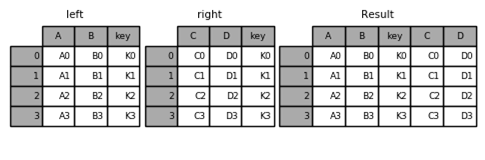
数据合并：拼接（concatenate）、连接（join）
数据拼接：
pd.concat([df1,df2,df3])
pd.concat([df1,df2,df3], keys=['a','b','c'])
pd.concat([df1,df2,df3], axis=1)
pd.concat([df1,df2,df3], ignore_index=True)
df1.append(df2)
数据连接：
pd.merge(df1, df2, on='key')
pd.merge(df1, df2, on=['key1','key2'])
pd.merge(df1, df2, on='key', how='inner')
inner、outer、left、right

Matplotlib

Matplotlib是一个强大的Python绘图和数据可视化的工具包。

• 安装方法：pip install matplotlib
• 引用方法：import matplotlib.pyplot as plt
• 绘图函数：plt.plot()
• 显示图像：plt.show()

一、plot函数

plot函数：绘制折线图
线型linestyle（-,-.,--,..）
点型marker（v,^,s,*,H,+,x,D,o,…）
颜色color（b,g,r,y,k,w,…）

plot函数绘制多条曲线
pandas包对plot的支持

二、图像标注

设置图像标题：plt.title()
设置x轴名称：plt.xlabel()
设置y轴名称：plt.ylabel()
设置x轴范围：plt.xlim()

设置y轴范围：plt.ylim()
设置x轴刻度：plt.xticks()
设置y轴刻度：plt.yticks()
设置曲线图例：plt.legend()

三、画布与子图

画布：figure
fig = plt.figure()
图：subplot
ax1 = fig.add_subplot(2,2,1)
调节子图间距：
subplots_adjust(left, bottom, right, top, wspace, hspace)

四、支持的图类型

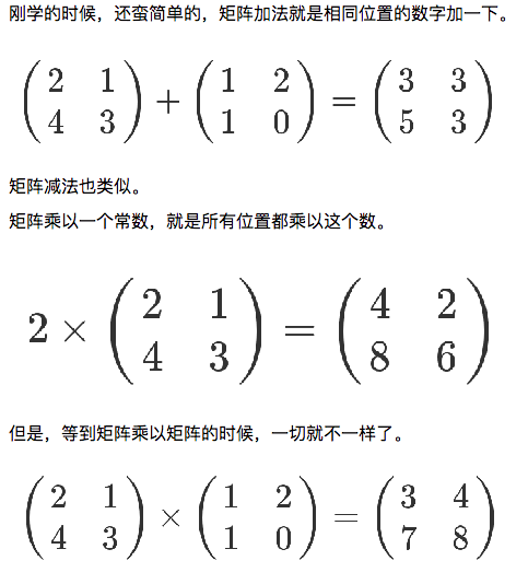
import matplotlib.pyplot as plt
import numpy as np
import pandas as pd
# plt.plot([1,2,3,4],[2,3,1,7])#折线图,x轴，y轴
# plt.plot([1,2,3,4],[2,3,1,7],"o") # "o"小圆点
# plt.plot([1,2,3,4],[2,3,1,7],"o-")# "o-"小圆点加折线实线
# plt.plot([1,2,3,4],[2,3,1,7],"o--")# "o-"小圆点加折线虚线
plt.plot([1,2,3,4],[2,3,1,7],"o--",color='red',label='Line A')# "o-"小圆点加折线虚线
plt.plot([1,2,3,7],[3,5,6,9],marker='o',color='black',label='Line B')
plt.title("Matplotlib Test Plot")
plt.xlabel("Xlabel")
plt.ylabel("Ylabel")
plt.xlim(0,5) #设置x轴的范围
plt.ylim(0,10)
plt.xticks([0,2,4])#x轴的刻度
plt.xticks(np.arange(0,11,2))
plt.xticks(np.arange(0,11,2),['a','b','c','d','e','f'])
plt.legend()#配合plot中的label='Line A' 一起使用
plt.show()


df=pd.read_csv('601318.csv',parse_dates=['date'],index_col='date')[['open','close','high','low']]
df.plot() #索引列直接变成X轴
plt.show()


x=np.linspace(-1000,1000,10000)
y1=x
y2=x**2
y3=3*x**3+5*x**2+2*x+1
plt.plot(x,y1,color='red',label="Line y=x")
plt.plot(x,y2,color='blue',label="Line y=x^2")
plt.plot(x,y3,color='black',label="Line y=3x^3+5x^2+2x+1")
plt.legend()
plt.xlim(-1000,1000)
plt.ylim(-1000,1000)
plt.show()


#####################画布
fig=plt.figure()
ax1=fig.add_subplot(2,2,1)  #画布分成2行2列 它占第一个位置
ax1.plot([1,2,3,4],[2,3,1,7])
plt.show()


fig=plt.figure()
ax1=fig.add_subplot(2,1,1)
ax1.plot([1,2,3,4],[2,3,1,7])

fig=plt.figure()
ax1=fig.add_subplot(2,1,2)
ax1.plot([1,2,3,4],[2,3,1,7])

#####################柱状图
plt.bar([0,1,2,4],[5,6,7,8])
plt.show()


data=[32,48,21,100]
labels=['Jan','Feb','Mar','Apr']
# plt.bar(np.arange(len(data)),data,color='red',width=0.3)
plt.bar(np.arange(len(data)),data,color='red',width=[0.1,0.2,0.3,0.4])
plt.xticks(np.arange(len(data)),labels=labels)
plt.show()


#####################饼图
plt.pie([10,20,30,40],labels=['a','b','c','d'],autopct="%.2f%%",explode=[0.1,0,0.1,0])
plt.axis('equal')
plt.show()

#####################K线图
import matplotlib.finance as fin
from matplotlib.dates import date2num
df=pd.read_csv('601318.csv',parse_dates=['date'],index_col='date')[['open','close','high','low']]
df['time']=date2num(df.index.to_pydatetime())
fig=plt.figure()
ax=fig.add_subplot(1,1,1)
arr=df[['time','open','close','high','low']].values
fin.candlestick_ochl(ax,arr)
fig.grid()
fig.show()

五、绘制K线图

matplotlib.finanace子包中有许多绘制金融相关图的函数接口。
绘制K线图：matplotlib.finance.candlestick_ochl函数

Tushare

• Tushare是一个免费、开源的python财经数据接口包。点击
• 安装：pip3 install tushare

"""
什么是数据分析
    是把隐藏在一些看似杂乱无章的数据背后的信息提炼出来，总结出所研究对象的内在规律
        使得数据的价值最大化
            分析用户的消费行为
            制定促销活动的方案
            制定促销时间和粒度
            计算用户的活跃度
            分析产品的回购力度
        分析广告点击率
            决定投放时间
            制定广告定向人群方案
            决定相关平台的投放
            ......
数据分析是用适当的方法对收集来的大量数据进行分析，帮助人们做出判断，以便采取适当的行动
    保险公司从大量赔付申请数据中判断哪些为骗保的可能
    支付宝通过从大量的用户消费记录和行为自动调整花呗的额度
    短视频平台通过用户的点击和观看行为数据针对性的给用户推送喜欢的视频


为什么学习数据分析
    有岗位的需求
        数据竞赛平台
    是Python数据科学的基础
    是机器学习课程的基础
数据分析实现流程
    提出问题
    准备数据
    分析数据
    获得结论
    成果可视化


开发环境介绍
anaconda
    官网：https://www.anaconda.com/
    集成环境：集成好了数据分析和机器学习中所需要的全部环境
    注意：
        安装目录不可以有中文和特殊符号
jupyter
    jupyter就是anaconda提供的一个基于浏览器的可视化开发工具
jupyter的基本使用
    启动：在终端中录入：jupyter notebook的指令，按下回车
    新建：
    python3：anaconda中的一个源文件
    cell有两种模式：
    code：编写代码
    markdown：编写笔记
    快捷键：
    添加cell：a或者b
    删除：x
    修改cell的模式：
    m：修改成markdown模式
    y：修改成code模式
    执行cell：
    shift+enter
    tab：自动补全
    代开帮助文档：shift+tab

数据分析三剑客
    numpy
    pandas(重点)
    matplotlib
"""


"""
numpy模块
NumPy(Numerical Python) 是 Python 语言中做科学计算的基础库。重在于数值计算，也是大部分Python科学计算库的基础，多用于在大型、多维数组上执行的数值运算。
numpy的创建
    使用np.array()创建
    使用plt创建
    使用np的routines函数创建
    
    

使用array()创建一个一维数组
import numpy as np
arr = np.array([1,2,3])
arr
array([1, 2, 3])

使用array()创建一个多维数组
arr = np.array([[1,2,3],[4,5,6]])
arr
array([[1, 2, 3],
       [4, 5, 6]])
       
数组和列表的区别是什么？
数组中存储的数据元素类型必须是统一类型
优先级：
字符串 > 浮点型 > 整数
arr = np.array([1,2.2,3])
arr
array([1. , 2.2, 3. ])

将外部的一张图片读取加载到numpy数组中，然后尝试改变数组元素的数值查看对原始图片的影响
import matplotlib.pyplot as plt
img_arr = plt.imread('./1.jpg')#返回的数组，数组中装载的就是图片内容
plt.imshow(img_arr)#将numpy数组进行可视化展示
<matplotlib.image.AxesImage at 0x117fb1b38>

img_arr = img_arr - 100 #将每一个数组元素都减去100
plt.imshow(img_arr)
<matplotlib.image.AxesImage at 0x1181a6b38>


zero()
ones()
linespace()
arange()
random系列
np.ones(shape=(3,4))

array([[1., 1., 1., 1.],
       [1., 1., 1., 1.],
       [1., 1., 1., 1.]])
       
np.linspace(0,100,num=20) #一维的等差数列数组
array([  0.        ,   5.26315789,  10.52631579,  15.78947368,
        21.05263158,  26.31578947,  31.57894737,  36.84210526,
        42.10526316,  47.36842105,  52.63157895,  57.89473684,
        63.15789474,  68.42105263,  73.68421053,  78.94736842,
        84.21052632,  89.47368421,  94.73684211, 100.        ])
        
np.arange(10,50,step=2) #一维等差数列
array([10, 12, 14, 16, 18, 20, 22, 24, 26, 28, 30, 32, 34, 36, 38, 40, 42,
       44, 46, 48])
       
np.random.randint(0,100,size=(5,3))
array([[19,  0, 17],
       [72, 29, 13],
       [69, 59, 68],
       [63, 54, 87],
       [70, 64,  0]])
       
numpy的常用属性
shape
ndim
size
dtype

arr = np.random.randint(0,100,size=(5,6))
arr
array([[43, 96, 75,  1, 34, 88],
       [96,  2, 17, 34, 26, 57],
       [71, 36, 11, 11, 10, 29],
       [72, 46, 51,  4, 27, 75],
       [80, 42, 27, 55, 19, 43]])
       
arr.shape #返回的是数组的形状
(5, 6)
arr.ndim #返回的是数组的维度
2
arr.size #返回数组元素的个数
30
arr.dtype #返回的是数组元素的类型
dtype('int64')
type(arr) #数组的数据类型
numpy.ndarray
numpy的数据类型
array(dtype=?):可以设定数据类型
arr.dtype = '?':可以修改数据类型image.png

arr = np.array([1,2,3])
arr.dtype
dtype('int64')

#创建一个数组，指定数组元素类型为int32
arr = np.array([1,2,3],dtype='int32')
arr.dtype
dtype('int32')

arr.dtype = 'uint8' #修改数组的元素类型
arr.dtype
dtype('uint8')


numpy的索引和切片操作（重点）
索引操作和列表同理
arr = np.random.randint(1,100,size=(5,6))
arr
array([[69, 80,  7, 90, 31, 44],
       [37, 57, 26, 92, 91, 34],
       [13, 16, 93, 54, 87, 34],
       [ 5, 16, 47, 66, 51, 12],
       [54, 63, 20, 11, 94, 88]])
       
arr[1]  #取出了numpy数组中的下标为1的行数据
array([37, 57, 26, 92, 91, 34])

arr[[1,3,4]] #取出多行
array([[37, 57, 26, 92, 91, 34],
       [ 5, 16, 47, 66, 51, 12],
       [54, 63, 20, 11, 94, 88]])
       
       
切片操作
    切出前两列数据
    切出前两行数据
    切出前两行的前两列的数据
    数组数据翻转


#切出arr数组的前两行的数据
arr[0:2] #arr[行切片]
array([[69, 80,  7, 90, 31, 44],
       [37, 57, 26, 92, 91, 34]])
#切出arr数组中的前两列
arr[:,0:2] #arr[行切片,列切片]
array([[69, 80],
       [37, 57],
       [13, 16],
       [ 5, 16],
       [54, 63]])
       
       
#切出前两行的前两列的数据
arr[0:2,0:2]
array([[69, 80],
       [37, 57]])
arr
array([[69, 80,  7, 90, 31, 44],
       [37, 57, 26, 92, 91, 34],
       [13, 16, 93, 54, 87, 34],
       [ 5, 16, 47, 66, 51, 12],
       [54, 63, 20, 11, 94, 88]])
#将数组的行倒置
arr[::-1]
array([[54, 63, 20, 11, 94, 88],
       [ 5, 16, 47, 66, 51, 12],
       [13, 16, 93, 54, 87, 34],
       [37, 57, 26, 92, 91, 34],
       [69, 80,  7, 90, 31, 44]])
#将数组的列倒置
arr[:,::-1]
array([[44, 31, 90,  7, 80, 69],
       [34, 91, 92, 26, 57, 37],
       [34, 87, 54, 93, 16, 13],
       [12, 51, 66, 47, 16,  5],
       [88, 94, 11, 20, 63, 54]])
#所有元素倒置
arr[::-1,::-1]
array([[88, 94, 11, 20, 63, 54],
       [12, 51, 66, 47, 16,  5],
       [34, 87, 54, 93, 16, 13],
       [34, 91, 92, 26, 57, 37],
       [44, 31, 90,  7, 80, 69]])
#将一张图片进行左右翻转
img_arr = plt.imread('./1.jpg')
plt.imshow(img_arr)
<matplotlib.image.AxesImage at 0x1182c3b00>

img_arr.shape
(300, 450, 3)
plt.imshow(img_arr[:,::-1,:]) #img_arr[行，列，颜色]
<matplotlib.image.AxesImage at 0x11835cb70>

#图片上下翻转
plt.imshow(img_arr[::-1,:,:])
<matplotlib.image.AxesImage at 0x118437ef0>

#图片裁剪的功能
plt.imshow(img_arr[66:200,78:300,:])
<matplotlib.image.AxesImage at 0x1187fee48>

变形reshape
arr#是一个5行6列的二维数组
array([[69, 80,  7, 90, 31, 44],
       [37, 57, 26, 92, 91, 34],
       [13, 16, 93, 54, 87, 34],
       [ 5, 16, 47, 66, 51, 12],
       [54, 63, 20, 11, 94, 88]])
#将二维的数组变形成1维
arr_1 = arr.reshape((30,))
#将一维变形成多维
arr_1.reshape((6,5))
array([[69, 80,  7, 90, 31],
       [44, 37, 57, 26, 92],
       [91, 34, 13, 16, 93],
       [54, 87, 34,  5, 16],
       [47, 66, 51, 12, 54],
       [63, 20, 11, 94, 88]])
       
级联操作
- 将多个numpy数组进行横向或者纵向的拼接
axis轴向的理解
    0:列
    1:行
问题：
    级联的两个数组维度一样，但是行列个数不一样会如何？
    
np.concatenate((arr,arr),axis=1)
array([[69, 80,  7, 90, 31, 44, 69, 80,  7, 90, 31, 44],
       [37, 57, 26, 92, 91, 34, 37, 57, 26, 92, 91, 34],
       [13, 16, 93, 54, 87, 34, 13, 16, 93, 54, 87, 34],
       [ 5, 16, 47, 66, 51, 12,  5, 16, 47, 66, 51, 12],
       [54, 63, 20, 11, 94, 88, 54, 63, 20, 11, 94, 88]])
arr_3 = np.concatenate((img_arr,img_arr,img_arr),axis=0)
plt.imshow(arr_3)
<matplotlib.image.AxesImage at 0x118f459b0>


常用的聚合操作
sum,max,min,mean
arr
array([[69, 80,  7, 90, 31, 44],
       [37, 57, 26, 92, 91, 34],
       [13, 16, 93, 54, 87, 34],
       [ 5, 16, 47, 66, 51, 12],
       [54, 63, 20, 11, 94, 88]])
arr.sum(axis=1)
array([321, 337, 297, 197, 330])
arr.max(axis=1)
array([90, 92, 93, 66, 94])


常用的数学函数
NumPy 提供了标准的三角函数：sin()、cos()、tan()
numpy.around(a,decimals) 函数返回指定数字的四舍五入值。
参数说明：
a: 数组
decimals: 舍入的小数位数。 默认值为0。 如果为负，整数将四舍五入到小数点左侧的位置
np.sin(2.5)
0.5984721441039564
np.around(3.84,2)
3.84


常用的统计函数
    numpy.amin() 和 numpy.amax()，用于计算数组中的元素沿指定轴的最小、最大值。
    numpy.ptp():计算数组中元素最大值与最小值的差（最大值 - 最小值）。
    numpy.median() 函数用于计算数组 a 中元素的中位数（中值）
    标准差std():标准差是一组数据平均值分散程度的一种度量。
    公式：std = sqrt(mean((x - x.mean())**2))
    如果数组是 [1，2，3，4]，则其平均值为 2.5。 因此，差的平方是 [2.25,0.25,0.25,2.25]，并且其平均值的平方根除以 4，即 sqrt(5/4) ，结果为 1.1180339887498949。
    方差var()：统计中的方差（样本方差）是每个样本值与全体样本值的平均数之差的平方值的平均数，即 mean((x - x.mean())** 2)。换句话说，标准差是方差的平方根。
arr[1].std()
26.66718749491384
arr[1].var()
711.138888888889


矩阵相关
    NumPy 中包含了一个矩阵库 numpy.matlib，该模块中的函数返回的是一个矩阵，而不是 ndarray 对象。一个 的矩阵是一个由行（row）列（column）元素排列成的矩形阵列。
    numpy.matlib.identity() 函数返回给定大小的单位矩阵。单位矩阵是个方阵，从左上角到右下角的对角线（称为主对角线）上的元素均为 1，除此以外全都为 0。

#eye返回一个标准的单位矩阵
np.eye(6)
array([[1., 0., 0., 0., 0., 0.],
       [0., 1., 0., 0., 0., 0.],
       [0., 0., 1., 0., 0., 0.],
       [0., 0., 0., 1., 0., 0.],
       [0., 0., 0., 0., 1., 0.],
       [0., 0., 0., 0., 0., 1.]])
转置矩阵
.T
arr.T
array([[69, 37, 13,  5, 54],
       [80, 57, 16, 16, 63],
       [ 7, 26, 93, 47, 20],
       [90, 92, 54, 66, 11],
       [31, 91, 87, 51, 94],
       [44, 34, 34, 12, 88]])

矩阵相乘
numpy.dot(a, b, out=None)
a : ndarray 数组
b : ndarray 数组
image.png

第一个矩阵第一行的每个数字（2和1），各自乘以第二个矩阵第一列对应位置的数字（1和1），然后将乘积相加（ 2 x 1 + 1 x 1），得到结果矩阵左上角的那个值3。也就是说，结果矩阵第m行与第n列交叉位置的那个值，等于第一个矩阵第m行与第二个矩阵第n列，对应位置的每个值的乘积之和。
线性代数基于矩阵的推导：
https://www.cnblogs.com/alantu2018/p/8528299.html

a1 = np.array([[2,1],[4,3]])
a2 = np.array([[1,2],[1,0]])
np.dot(a1,a2)
array([[3, 4],
       [7, 8]])

"""