Local dimming algorithm in matlab

LED局部背光算法的matlab仿真 

       最近公司接了华星光电（TCL）的一个项目LCD-BackLight-Local-Diming-Algorithm-IP ，由于没有实际的硬件，只能根据客户给的论文 算法进行调研，评估和确认。即先理解论文的算法，再用MATLAB或OpenCV仿真，再通过视觉或客观图像评价指标评估算法效果，最后通过对几种论文算法的实验仿真效果分析比较确定一种算法，作为fpga实现。最大感触是得搞清楚实际情况再行动！

一  论文算法原理

     论文题目为<< Backlight Local Dimming Algorithm for High Contrast LCD-TV>>，我一般看英语论文先用excel表格记录论文编号，题目，背景，关键词，主要方法，缺点（可以创新的地方），结论等核心点，接着看文献顺序为：摘要，结论，实验，着重看论文算法（准确理解，很耗时），若很闲则会看Introduction。当然，这次对这个算法的改进是多次，每次蹦出一个想法就改善算法，主要有三点：一是多用参数化定义，提高算法移植性和通用性。二是多想办法减少重复劳动，如在一个窗口中一次显示多个参数取不同值的结果，这一点很重要，以后多用。三是，一个算法的改进周期很长，直接方法是看高手的写法，而且得多次对比和看文档书籍才有提升，而不是成谜自己的小成果。

下面直接给出算法整体框架：

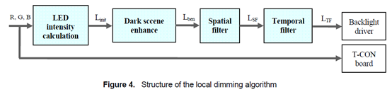
 从上图可以看出整个算法分为四步，LED亮度强度计算，暗区域增强，空间滤波器，时间滤波器。注意点1：算法的仿真是放在FPGA上通过对LED的亮度调节，即整个算法是对LED块的分块的亮度进行处理，由于没有LED等实际硬件，本次仿真是对图像分块后的每个图像块亮度强度进行处理。注意点2：算法的实验是进行视频仿真，而MATLAB主要是进行图像处理，故本次时间滤波器的处理，这一步包含当前帧和上一帧，通过用potplayer软件截取一帧视频图像，方法如下：

第一步是视频素材下载网站：

视频下载网站（水印）
https://www.vjshi.com/watch/6162152.html
视频素材下载（无水印）
https://mixkit.co/free-stock-video/nature/

第二步是PotPlayer的截取视频的一帧图像：在用potpalyer播放视频时，快捷键crtl+G打开连续截取画面，按照下面的12345步骤即可成功截取想要的两帧图像。

 

论文算法的参数如下表格所示：

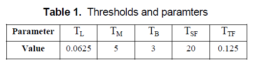
 上面的参数在第一步到第三步都会有所涉及，这里提前给出。

（一）LED亮度强度计算

1.算法介绍

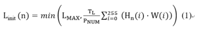
 Linit(n)为第n个LED块的初始亮度强度，第一步的输出；LMAX可允许的最大LED亮度强度水平；TL 是一个预定义参数，用来控制局部调节水平，由表1可知为0.0625；P_NUM（第n个图像块的总像素数量）；

 Hn(i)是第n个图像块的直方图；W(i)是预定义的权重向量，论文里为变量i的平方。

2.MATLAB代码实现

从上面公式1可知，算法整体为两项中取最小值，第二项有点繁琐，那就从第二项开始：第二项的TL，Pnum都很好计算，一个为常数0.0625，一个为图像块的总像素数，即图像的尺寸M*N，图像行列的乘积；

第二项中的图像块直方图和权重W(i)的乘积的累加和需注意，图像块的直方图怎么实现，若是调用imhist仅仅是显示直方图，而在这里明显不对，故需要查资料弄懂图像的直方图的含义，通过看<<数字图像处理>>这本书，明白图像的直方图：对应灰度级的像素数。而MATLAB怎么表示，通过在MATLAB中搜索help imhist和不断看相关函数发现了histogram函数。在MATLABhelp文档中，知道了一种用法可以表示图像某个灰度级的像素数：h = histogram(In,256);counts=h.Values ;通过这两行代码把第n个图像块的直方图搞定了，那么公式1则轻松表示出来了。故对公式1的处理关键：拆分，弄明白直方图的含义，通过经典的数字图像处理书籍和matlab官方的文档，准确理解直方图含义。由于后面的步骤要调用这个结果，故把这一步封装成函数，调用很方便。代码如下：

function L_init = Linit(In)
[m,n]=size(In);
 num_p=m*n;
    s=0;
    h = histogram(In,256);
counts=h.Values  ;
    for i2 = 1:256
        h = counts(i2);
       ii= i2^2;
   s=s+(h*ii); %求得所有像素与灰度级平方的乘积。
  % s=s+(h*i2);
    end
 num_p = double (num_p);
  s = double (s);
L_temp=(0.0625/num_p)*s;
L_init = min(63,L_temp);
end

（二）暗区域增强

通过第一步的matlab代码实现，我们可以学会MATLAB编写方法：第一对公式的每个变量准备理解，如最大值，像素总数，灰度级，权重变量。第二对公式拆分，把握关键的一点，即难一点实现的，如上面的直方图。三是查阅权威书籍<<数字图像处理>>和matlab官方文档，弄懂直方图的实现，再把算法完整编写。对于这一步的暗区域增强，实现过程相似。

1.算法介绍

 Lben 是增强的LED亮度强度灰度；L_mean 是当前图像的所有图像块的 L_init的平均值；T_M用来定义暗区域的阈值；T_B用来控制暗区域增强水平的预定义参数；

2.MATLAB代码实现

     通过上面的分析可知，L_init的使用通过调用第一步的函数输出值即可，而L_mean 的计算则需要注意，它是包含图像的所有块的L_init的均值，故需要用一个矩阵存放所有图像块的L_init的值，再用matlab的mean2函数即可，而后面的T_M，T_B用通过表格可知分别是5和3。整体是选择结构，用matlab的if语句实现即可。

function L_ben = Lben(Lini,L_mean)
TM = 5;
if(Lini<L_mean | TM<L_mean) % L_mean = 20
    L_ben = Lini;
else
     L_ben =min(63 ,Lini+3*(Lini-L_mean));
end
end

（三）空间滤波器处理

1.算法介绍

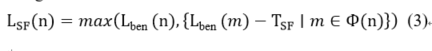
 LSF(n)是第n个LED块的亮度强度的空间滤波器的输出；TSF 是用来平滑滤波器的预定义参数；Φ(n)是大小为3X3的第n个块的邻域中心；这一步的关键是对3*3的领域空间的理解，以第n块为中心，共3*3总共为9个图像块的领域。这个领域用一个3*3的矩阵索引实现，即Lben(m)是领域中每一块的 Lben 值。

2.MATLAB代码实现

其实关键点就是3*3的邻域实现，我的想法是，将10*10的Lben最外围全部舍掉，即行和列范围都是2-9，然后舍掉本身即第n块的Lben，这总共8个元素，构成一个数组，取数组的最大值和第n块的Lben比较取较大值，得到空间滤波器的输出，每一块都能得到一个输出。思路的代码如下：

function L_SF = S_filter(LSF_ini,temp_Lben,T_SF)
%function L_SF = S_filter(LSF_ini,T_SF)
temp_Lsf = temp_Lben;
[row,col]=size(temp_Lben);
LSF_temp1=zeros(1,9);
for nx=2:row-1
    for ny=2:col-1
       % 取出对应需要进行运算区域的数据
        LSF_temp1 = temp_Lsf(nx-1:nx+1,ny-1:ny+1);
       % convert to 
        temp11=[LSF_temp1(1,:),LSF_temp1(2,1),LSF_temp1(2,3),LSF_temp1(3,:),];
       % 赋值
        temp_max =  max(temp11);
    end
end
Len_nn = LSF_ini;
       L_SF = max(Len_nn,temp_max-T_SF);
end

 (四) 时间滤波

1.算法介绍

LTF(n)是时间滤波器的输出；(k) 和 (k-1)指当前帧和前一帧；R (0<R ≤1)为控制IIR低通滤波器的平滑程度的参数。

其中，R由视频内容自适应决定，其表达式如下：

TTF 用来控制IIR滤波器形状的预定义参数，为0.125。Pmean整个图像的归一化平均像素值。

2.MATLAB代码实现

时间滤波由上面两个公式(4)(5)组成，包含两个部分，即第一步(5)是公式(4)中的R，故我们可以先编写matlab函数实现R，再带入公式(4)；第二步LSF为空间滤波的输出，可以封装为一个函数；在顶层调用这两部分的函数即可实现公式(4)的功能。

       R的代码，第一步是计算两帧图像的归一化平均像素值，两帧图像这里为上面用potplayer软件截取的视频图像，归一化平均像素值那么需要用到归一化函数 normalize，还有平均值函数mean和最小值函数min,按照公式(4)直接敲即可：

%calculate the result of R in EQ.(4) for algorithm
%the input is two frame of image
%the output is R in EQ.(4)
function R_S4 = cal_R(IMA,IMA1)
%RGB = imread('../pic/EE01000_1000.jpeg');%1000*1000 pixel of image
%RGB1 = imread('../pic/EE4_1000.jpeg');%1000*1000 pixel of EE4_1000.jpeg
%THE RESULT OF above ima is R = 0.4626
%RGB = imread('ee0_1000.jpg');%1000*1000 pixel of image
I =rgb2gray(IMA);
I1 =rgb2gray(IMA1);
%normalize the pixel of ima
I = double(I);
I1 = double(I1);
I_nr=normalize(I,'range');
I1_nr = normalize(I1,'range');
 Pmean0 = mean(I_nr,'all');%the normalize mean of previous frame
  Pmean1 = mean(I1_nr,'all');%the normalize mean of current frame
  R_S4_temp = 0.125+Pmean0+Pmean1;
  R_S4 = min(1,R_S4_temp);%the parameter R of step4 for algorithm
end

　公式(4)还调用了第三步的公式(3)空间滤波的输出，故我们可以把第三步空间滤波的输出封装成一个函数如下所示，在时间滤波这一步直接调用即可：

%main function begin
function Lsf_out = cal_Lsf(image)
tic;
RGB = image;
%RGB = imread('ee0_1000.jpg');%1000*1000 pixel of image
%parameter
global ima_width;
global ima_hight;
global block_width;
global block_hight;
global block_num_h;
global block_num_v;
%parameter
%I =rgb2gray(RGB);
%normalize the pixel of ima
%---Table 1. Thresholds and paramters----
global Y_M;
Y_M = 230;%the most bright scene
global T_L;
% T_L = 0.025;
%T_L is a predefined parameter 
%-used to control the local dimming degree
global T_M;
T_M = 18;%the most dark scene
global T_B;
T_B = 3;
global T_SF;
T_SF = 120;

%----Table 1. Thresholds and paramters---
IMA_YCBCR = rgb2ycbcr(RGB);
Y=IMA_YCBCR(:,:,1);
% figure 
% imshow(I);
 temp_Linit = zeros(block_num_v,block_num_h);
% % I1 = rgb2gray(I);
t_row =  0:block_hight:ima_hight;   % the row'coordinates of each block
t_row1= t_row;
t_row = t_row+1;%pattention-->reduced add the Extra 1
t_col = 0:block_ima_width;   % the column'coordinates of each block
t_col1= t_col;
t_col = t_col+1;
% % save space to predifine variable
% %temp = repmat(int8(0), 100, 100);%arry cannot deliver to point
temp1 = cell(block_num_v,block_num_h);% creat cell struct
        %the number of block in row or column
for i = 1 : block_num_v
    for j = 1 : block_num_h
        temp = Y(t_row(i):t_row1(i+1), t_col(j):t_col1(j+1));
        temp1{i,j}=temp;
        In =  temp1{i,j};
        temp_Linit(i,j)= Linit(In);
 %subplot(10, 10, 10*(i-1)+j); imshow(temp);
    end
end
% %%cal L_ben by cycle
% 
L_mean = mean2(temp_Linit);
 temp_Lben = zeros(block_num_v,block_num_h);
for i1 = 1 : block_num_v
    for j1 = 1 : block_num_h
        Lben_In =   temp_Linit(i1,j1);
        temp_Lben(i1,j1)= Lben(Lben_In,L_mean);
    end
end
% %%combine L_SF to arry
%T_SF = 20;
 temp_Lsf = zeros(block_num_v,block_num_h);
for i4 = 1 : block_num_v
    for j4 = 1 : block_num_h
        Lsf_In =   temp_Lben(i4,j4);
        temp_Lsf(i4,j4)= S_filter(Lsf_In,temp_Lben);
    end
end
% 
% %YCBCR1_temp{i,j}=temp_Lsf(i,j);
Lsf_out = temp_Lsf;
end
%main function end

% %CONTINU TO l_init, L_ben,L_sf
function L_init = Linit(In)
global Y_M;
global T_L;

[m,n]=size(In);
 num_p=m*n;
    s=0;
   % h = histogram(In,256);
%counts=h.Values  ;
counts = imhist(In,256);
    for i2 = 1:256
        h = counts(i2);
       ii= (i2-1)^2;
   s=s+(h*ii); %求得所有像素与灰度级平方的乘积。
  % s=s+(h*i2);
    end
 num_p = double (num_p);
  s = double (s);
L_temp=(T_L/num_p)*s;
L_init = min(Y_M,L_temp);
end
% % %part 2 the enhance method
function L_ben = Lben(Lini,L_mean)
global T_M;
global Y_M;
global T_B;
if(Lini<L_mean | T_M<L_mean) % L_mean = 20
    L_ben = Lini;
else
     L_ben =min(Y_M ,Lini+T_B*(Lini-L_mean));
end
end
% % %part 3 the Spatial filter 
% rng(0,'twister');%初始化随机数生成器
% a = 1;
% b = 64;
% rr = (b-a).*rand(16,1) + a;%creat a rand matrix 
% LSF=reshape(rr,4,4);
% %contains 16 datas the value range from 1 to 64
% for i = 1:4
%     for j = 1:4
%         LSF_i= LSF(i,j);
%         ll = S_filter(LSF_i,i,j,20);
%     end
% end
function L_SF = S_filter(LSF_ini,temp_Lben)
%function L_SF = S_filter(LSF_ini,T_SF)
global T_SF;
temp_Lsf = temp_Lben;
[row,col]=size(temp_Lben);
LSF_temp1=zeros(1,9);
for nx=2:row-1
    for ny=2:col-1
       % 取出对应需要进行运算区域的数据
        LSF_temp1 = temp_Lsf(nx-1:nx+1,ny-1:ny+1);
       % convert to 
        temp11=[LSF_temp1(1,:),LSF_temp1(2,1),LSF_temp1(2,3),LSF_temp1(3,:),];
       % 赋值
        temp_max =  max(temp11);
    end
end
Len_nn = LSF_ini;
       L_SF = max(Len_nn,temp_max-T_SF);
end


%设置循环，对每个像素进行八邻域中值运算
%设置循环条件

如上面代码所示，含有全局参数，这是增加代码的移植性和通用性，即简单改参数就能仿真不同输入和条件下的图像效果。

二 主函数的设计

   （一）时间滤波的顶层函数

由于这个LED的局部调光算法的核心思想：

根据图像的内容分块，以及对不同块使用不同的系数（图像块或LED块的亮度强度）去调节背光（达到高对比度，即亮的地方更亮，暗的地方更暗）。

上面是我对LED局部调光算法的总结。故要想实现这个算法，得搞定怎么对图像分块，用MATLAB表示第n块图像，对第n块图像实现上面的（一）（二）（三）步处理，这是难点。我刚开始直接想的是MATLAB现成的函数：B = blockproc(A,[m n],fun)函数。但这个函数的输入为原图像，输出直接和原图同大小的一幅图像，不能实现我们想要的第n块图像。我在这卡了很久，通过大量查阅官网的图像分块资料和看数字图像处理书籍，及网上查阅csdn博客和MATLAB中文论坛，终于找到办法：即数字图像就是一个多维矩阵，像素点对应矩阵元素，故图像分块就是矩阵的分块。如本文的图像分块为10*10共100块，输入图像分辨率大小为1000*1000的rgb图像，则每一图像块为100*100的矩阵。我们把这个100*100的矩阵赋值给一个10*10的元胞数组的一个元素（关键，由于矩阵不能赋值给一点），然后把元胞数组的元素赋值给临时变量temp，这个大小为100*100的矩阵temp就是第n块的图像块，再传递给上面的函数调用即可。当然，针对10*10共100块的图像块处理，会频繁用到for循环结构，幸亏上面把每一步封装成函数，我们调用即可，不然很难搞。做matlab算法和FPGA的设计一样，都是循序渐进，即模块化设计（一个功能一个函数），把每个模块仿真实现无误后，再顶层调用即可。为了提高算法的通用性，可以把图像的宽和高等参数，表示为一个参数，以后输入不同分辨率图像直接修改参数即可，本次就省略哦。LED局部调光算法的主函数如下：

%calculate the luminous of rgb ima by the whole algorithm
%display the modified luminous of rgb image
%input image
%output the modified luminous of RGB image
%date 08.04
close all
clear
clc;
%load('S1.mat');
tic;
% %blockproc  
% 
% % myfun = @(block_struct) block_struct.data;
% %I = imread('e1.jpeg');%100*100 pixel of image
% RGB = imread('../pic/meadowP1000_1000.jpg');%1000*1000 pixel of image previous frame
% RGB1 = imread('../pic/meadowC1000_1000.jpg');%1000*1000 pixel 
% RGB = imread('../pic/fireworksP1000_1000.jpg');%1000*1000 pixel of image previous frame
% RGB1 = imread('../pic/fireworksC1000_1000.jpg');%1000*1000 pixel 
RGB = imread('../pic/moonP1000_1000.jpg');%1000*1000 pixel of image previous frame
RGB1 = imread('../pic/moonC1000_1000.jpg');%1000*1000 pixel 
%RGB = imread('ee0_1000.jpg');%1000*1000 pixel of image
%calculate the R of between current frame and previous frame
R = cal_R(RGB,RGB1);
%calculate the Ltf of the Nth image blcok
temp_Lsf0 = cal_Lsf(RGB);%Lsf of previous frame
temp_Lsf1 = cal_Lsf(RGB1);
Ltf0 = R*temp_Lsf0;
Ltf1 = (R*temp_Lsf1)+((1-R)*Ltf0);%Ltf of current frame
temp_Lsf = Ltf1;
% %YCBCR1_temp{i,j}=temp_Lsf(i,j);
tt_row = 0:100:1000;   % the row'coordinates of each block
tt_row1= tt_row;
tt_row = tt_row+1;%pattention-->reduced add the Extra 1
tt_col = 0:100:1000;   % the column'coordinates of each block
tt_col1= tt_col;
tt_col = tt_col+1;
% % save space to predifine variable
% %temp = repmat(int8(0), 100, 100);%arry cannot deliver to point
YCBCR1_out = zeros(1000);
YCBCR1_temp = cell(10);% creat cell struct
len1 = 10;          %the number of block in row or column
for i5 = 1 : len1
    for j5 = 1 : len1
        YCBCR1_temp{i5,j5}=temp_Lsf(i5,j5);
   YCBCR1_out(tt_row(i5):tt_row1(i5+1), tt_col(j5):tt_col1(j5+1))=YCBCR1_temp{i5,j5};

 %subplot(10, 10, 10*(i-1)+j); imshow(temp);
    end
end
% figure
% imshow(RGB);title('RGB');
 YCBCR = rgb2ycbcr(RGB);
%   figure
%  imshow(YCBCR);title('YCBCR');
YCBCR(:,:,1)=YCBCR1_out;
OUT = ycbcr2rgb(YCBCR);
OUT1 = OUT + RGB;% comibine the original image and modified image
%OUT1 the output of
% figure
% imshow(OUT);title('OUT');
% figure
% imshow(OUT1);title('OUT1');
toc;
%离y轴距离，离x轴距离，子图宽，子图高
subplot('Position',[0.1 0.1 0.8 0.8]);imshow(RGB);title('RGB');
% [left bottom width height].
figure
subplot(1,3,1);imshow(RGB);title('RGB');
subplot(1,3,2); imshow(YCBCR);title('YCBCR');
subplot(1,3,3);imshow(OUT1);title('OUT1');
% % for m = 1:10
% %     for n = 1:10
% %         temp2=(temp1{m,n});
% %        subplot(10, 10, 10*(m-1)+n); imshow(temp2);    
% %     end
% % end
% %CONTINU TO l_init, L_ben,L_sf

%设置循环，对每个像素进行八邻域中值运算
%设置循环条件

当然，这里的代码就是公式(4)的顶层代码。

(二)高效的仿真手段

       回头看看最开始的（一 论文算法原理）Table 1表格，竟然五个参数！天啊，做实验恐怖得一周，要是手动一个个改。这种体力活一直都是这样搞的，这次想偷偷懒，没必要搞重复劳动。自然想到了，要是直接一次显示多个参数取不同值的结果，多爽哈！以前一周的实验，现在几分钟万事！哈哈，这就是效率。

怎么一次显示多个参数取不同值？

思路是：直接把算法封装成一个函数，用for循环遍历不同值，结合subplot和title函数，在一个窗口显示输入不同参数的对应图像。

1.简单例子1--直接上图：一次显示一个参数取四个不同值的图像效果

 上面这一个窗口，包含一个参数a取四个不同值的图像效果，这个简单的例子为图像增强的线性变换，这个线性变换的增强函数如下：

for a = 1:4
       out = a*RGB+0.5; 
subplot(2,2,a);imshow(out);
% title(sprintf(a,b));
%title(num2str(4*(a-1)+b));%one title display different images from 1 to 16 
title(num2str(a));%Create Multiline Title
end

　2 例子2为一次显示两个参数各取四个不同值的图像效果　

 如上图所示，一次显示参数a和b,一个为对比度增强系数，一个为亮度，两个参数在1到4之间取值的16中组合结果，代码如下：

for a = 1:4
    for b = 1:4
       out = a*RGB2+b; 
subplot(4,4,(4*(a-1)+b));imshow(out);
% title(sprintf(a,b));
%title(num2str(4*(a-1)+b));%one title display different images from 1 to 16 
title({num2str(a);num2str(b)});%Create Multiline Title
    end
end

　　可以看出关键为subplot的坐标和title中变量的写法。直接搜索相关函数文档理解。既然可以显示两个参数取不同值，自然能够推广到多个参数。

3 输入任意参数的用法（一次显示参数取多个不同值的结果）

在上面的两个例子中，我们为了着重设计思路，将参数取为1：4这种情况，但实际你会碰到参数取值30-50或者0.01到0.05这种不是从1开始或每次增加1.既然，一个参数，两个参数都会了，那么任意参数只需要转换为上面的两个例子即可，如下图的代码所示：

 上面的25张图像，为水平和垂直方向的分区数量的参数，各自取30：50到范围的仿真效果，MATLAB代码如下：

for block_num_v = 30:5:50
    for block_num_h = 30:5:50
        a =((block_num_v-30)/5)+1;
        b =((block_num_h-30)/5)+1;
       out = A1_Localdim_814(RGB,RGB1); 
subplot(5, 5, 5*(a-1)+b);imshow(out);
% title(sprintf(a,b));
%title(num2str(4*(a-1)+b));%one title display different images from 1 to 16 
title({num2str(block_num_v);num2str(block_num_h)});%Create Multiline Title
    end
end

　　可以看出，对于输入多个任意参数，用到数值转换：即把输入参数减去起点30，除以公差（数列），加上1就转换为我们的线性转换例子1和2。

注意点：在调用的子函数中，不能包含有画图相关的函数，如figure, subplot, imshow等，否则就会把参数不同取值的仿真结果分别显示在多个窗不同口中，如下图所示：

 那是在调用的函数GABF_DDE_top814中有下面几行代码：

figure;
subplot(1,1,1);
imshow(test_R);

相应的例子代码如下：

%this file is used to
%once display the result of Algorithm for 20 images
%pattention:the function can't have a figure
%--subplot(1,1,1);or imshow(test_R2); 
clc;
close all;
clear;
%----a example for display 4 images----
I = cell(2);
I{1,1}=load('../data/S1.mat','S');
I{1,2}=load('../data/S2.mat','S');
I{2,1}=load('../data/S3.mat','S');
I{2,2}=load('../data/S4.mat','S');

for i =1:2
    for j = 1:2
        temp_I = I{i,j};
        temp = temp_I.S;
        out = GABF_DDE_top814(temp);
        subplot(2,2,(2*(i-1)+j));
        imshow(out);title({num2str(i);num2str(j)});
    end
end
%----a example for display 4 images----
%extend to display 20 images

通过对实现一次显示参数取不同值的结果的分析，利用这个方法，我们就能极大的节省时间，偷个懒！

4 matlab的图像算法的结构

如上图所示，有三层结构，最顶层为仿真测试，其次为算法顶层，最后是功能函数。仿真测试顶层，用来做不同输入参数和不同输入图像的实验，如上面讲的参数取不同值的方法，输入不同分辨率图像，灰度图像，RGB图像等。算法顶层，即能够完整实现算法功能，核心就是能够封装成一个函数，实现算法的效果。如本次算法为LCD局部背光调节算法，就能够实现根据图像的内容，对一帧图像进行分块M*N块后，进行算法流程的四步处理后，达到预期的效果：即让亮的区域更亮，暗的区域更暗。从而提升视频图像对比度和亮度，输出高质量的视觉图像，给人更好的视觉体验。功能函数，对应于具体的算法步骤，如算法流程中第一步求初始亮度，空间滤波等，多个函数可以放在一个MATLAB文件里，也可以单独放一个文件。为了理解，冗余复杂的函数可以单独放一个文件，简单的函数多个放一起。

(一)测试顶层函数

%This file is used to 
%simulate A1_Localdim_814.m or verify it

%------------1000*1000 of ima-------------
% RGB = imread('../pic/meadowP1000_1000.jpg');%1000*1000 pixel of image previous frame
% RGB1 = imread('../pic/meadowC1000_1000.jpg');%1000*1000 pixel 
% RGB = imread('../pic/fireworksP1000_1000.jpg');%1000*1000 pixel of image previous frame
% RGB1 = imread('../pic/fireworksC1000_1000.jpg');%1000*1000 pixel 
RGB = imread('../pic/moonP1000_1000.jpg');%1000*1000 pixel of image previous frame
RGB1 = imread('../pic/moonC1000_1000.jpg');%1000*1000 pixel 
%------------1000*1000 of ima-------------
%------------1920*1080 of ima-------------
% RGB = imread('../pic/sunset_pre1920_1080.jpg');%1920*1080 pixel of image previous frame
% RGB1 = imread('../pic/sunset_current1920_1080.jpg');%1920*1080 pixel 
% RGB = imread('../pic/blinking_round_lights_pre1920_1080.jpg');
% RGB1 = imread('../pic/blinking_round_lights_cur1920_1080.jpg');
% RGB = imread('../pic/volumetric_pre1920_1080.jpg');%volumetric_pre1920_1080
% RGB1 = imread('../pic/volumetric_cur1920_1080.jpg');
RGB2 = imread('../pic/LYF2.jpg');
%------------1920*1080 of ima-------------
I = rgb2gray(RGB);
 YCBCR = rgb2ycbcr(RGB);
 YCBCR_Y =( YCBCR(:,:,1));
%   subplot(1,1,1);imshow(YCBCR_Y);title('YCBCR_Y');
%%test 1
%-------the result of different numbers of blocks for a ima-------------
%parameters
tic;
global block_num_h;
global block_num_v;
global T_L;
 T_L = 0.025;
% %---1000*1000 of ima----
%  block_num_v=50;
%  block_num_h=50;         %the number of block in the horizontal direction
% %---1000*1000 of ima----
%---1920*1080 of ima----the parameters is a multiple of 2
%block_num_h=64,32,16 or 8
%block_num_v=40,20,10
%  block_num_v=40;
%  block_num_h=64;         %the number of block in the horizontal direction
%---1000*1000 of ima----
%parameters
for block_num_v = 30:5:50
    for block_num_h = 30:5:50
        a =((block_num_v-30)/5)+1;
        b =((block_num_h-30)/5)+1;
       out = A1_Localdim_814(RGB,RGB1); 
subplot(5, 5, 5*(a-1)+b);imshow(out);
% title(sprintf(a,b));
%title(num2str(4*(a-1)+b));%one title display different images from 1 to 16 
title({num2str(block_num_v);num2str(block_num_h)});%Create Multiline Title
    end
end
%-------the result of different numbers of blocks for a ima-----------
%%test 2
%-------the result of different values of global T_L;-----------
% global T_L;
% for T_L = 0.01:0.005:0.05
%         a =((T_L-0.01)/0.005)+1;
%        out = A1_Localdim_814(RGB,RGB1); 
% subplot(3,3,a);imshow(out);
% % title(sprintf(a,b));
% %title(num2str(4*(a-1)+b));%one title display different images from 1 to 16 
% title(num2str(T_L));%Create Multiline Title
% end
%example--once display different values of parameter at the same figure
% for a = 1:4
%     for b = 1:4
%        out = a*RGB2+b; 
% subplot(4,4,(4*(a-1)+b));imshow(out);
% % title(sprintf(a,b));
% %title(num2str(4*(a-1)+b));%one title display different images from 1 to 16 
% title({num2str(a);num2str(b)});%Create Multiline Title
%     end
% end
%example
toc;

主要包含三个测试：一是在水平和垂直方向上不同分区数量的分块时的仿真效果。二是Table 1表格中T_B取不同值的仿真效果。三是上面分析的提高算法效率的例子，一次显示多个参数取不同值的仿真效果。

(二)算法顶层

%calculate the luminous of rgb ima by the whole algorithm
%display the modified luminous of rgb image
%input image
%output the modified luminous of RGB image
%date 08.12
%main work is adjust the parameters of Table 1
% close all
% clear
% clc;
%load('S1.mat');
function YCBCR1_out = A1_Localdim_814(RGB,RGB1)

% %blockproc  
% 
% % myfun = @(block_struct) block_struct.data;
%------------1000*1000 of ima-------------
% RGB = imread('../pic/meadowP1000_1000.jpg');%1000*1000 pixel of image previous frame
% RGB1 = imread('../pic/meadowC1000_1000.jpg');%1000*1000 pixel 
% RGB = imread('../pic/fireworksP1000_1000.jpg');%1000*1000 pixel of image previous frame
% RGB1 = imread('../pic/fireworksC1000_1000.jpg');%1000*1000 pixel 
% RGB = imread('../pic/moonP1000_1000.jpg');%1000*1000 pixel of image previous frame
% RGB1 = imread('../pic/moonC1000_1000.jpg');%1000*1000 pixel 
%------------1000*1000 of ima-------------
%------------1920*1080 of ima-------------
% RGB = imread('../pic/sunset_pre1920_1080.jpg');%1920*1080 pixel of image previous frame
% RGB1 = imread('../pic/sunset_current1920_1080.jpg');%1920*1080 pixel 
% RGB = imread('../pic/blinking_round_lights_pre1920_1080.jpg');
% RGB1 = imread('../pic/blinking_round_lights_cur1920_1080.jpg');
% RGB = imread('../pic/volumetric_pre1920_1080.jpg');%volumetric_pre1920_1080
% RGB1 = imread('../pic/volumetric_cur1920_1080.jpg');
%------------1920*1080 of ima-------------
I =rgb2gray(RGB);
I1 =rgb2gray(RGB1);
%% parameters...
%The horizontal direction---h
%The vertical direction---v
global ima_width;          %the number of column for image
global ima_hight;           %the number of row
global block_width;        %the number of column for a block
global block_hight;         %the number of row for a block
global block_num_h;
global block_num_v;

[ima_hight,ima_width]=size(I);
% block_num_v=40;
% block_num_h=64;         %the number of block in the horizontal direction

block_width = floor(ima_width/block_num_h);
block_hight = floor(ima_hight/block_num_v);
%% 
%calculate the R of between current frame and previous frame
global T_TF;
T_TF = 0.125;
R = cal_R(RGB,RGB1);
%calculate the Ltf of the Nth image blcok
temp_Lsf0 = cal_Lsf(RGB);%Lsf of previous frame
temp_Lsf1 = cal_Lsf(RGB1);
Ltf0 = R*temp_Lsf0;
Ltf1 = (R*temp_Lsf1)+((1-R)*Ltf0);%Ltf of current frame
temp_Lsf = Ltf1;
% %YCBCR1_temp{i,j}=temp_Lsf(i,j);
tt_row = 0:block_hight:ima_hight;   % the row'coordinates of each block
tt_row1= tt_row;
tt_row = tt_row+1;%pattention-->reduced add the Extra 1
tt_col = 0:block_ima_width;   % the column'coordinates of each block
tt_col1= tt_col;
tt_col = tt_col+1;
% % save space to predifine variable
% %temp = repmat(int8(0), 100, 100);%arry cannot deliver to point
YCBCR1_out = zeros(ima_hight,ima_width);
YCBCR1_temp = cell(block_num_v,block_num_h);% creat cell struct
          %the number of block in row or column
for i5 = 1 : block_num_v
    for j5 = 1 : block_num_h
        YCBCR1_temp{i5,j5}=temp_Lsf(i5,j5);
   YCBCR1_out(tt_row(i5):tt_row1(i5+1), tt_col(j5):tt_col1(j5+1))=YCBCR1_temp{i5,j5};

 %subplot(10, 10, 10*(i-1)+j); imshow(temp);
    end
end
% figure
% imshow(RGB);title('RGB');

%  figure
% subplot(1,2,1); imshow(YCBCR1_out);title('YCBCR1_out');
 YCBCR = rgb2ycbcr(RGB);
 YCBCR_Y =( YCBCR(:,:,1));
  %------min/max luminous--------
 %find the max luminous of ima
 %the min luminous
 Y_MAX = max(YCBCR_Y,[],'all');
 Y_MIN = min(YCBCR_Y,[],'all');
 %------min/max luminous--------
YCBCR1_out = uint8(YCBCR1_out);
%  figure
%  subplot(1,2,2); imshow(YCBCR1_out);title('YCBCR1_out');
% subplot(1,2,1);imshow(YCBCR_Y);title('YCBCR_Y');
%   figure
%  imshow(YCBCR);title('YCBCR');
% YCBCR(:,:,1)=YCBCR1_out;

% OUT = ycbcr2rgb(YCBCR);
% OUT1 = OUT + RGB;% comibine the original image and modified image
%OUT1 the output of
% figure
% imshow(OUT);title('OUT');
% figure
% imshow(OUT1);title('OUT1');

end
%离y轴距离，离x轴距离，子图宽，子图高
% subplot('Position',[0.1 0.1 0.8 0.8]);imshow(RGB);title('RGB');
% [left bottom width height].
% figure
% subplot(1,3,1);imshow(RGB);title('RGB');
% subplot(1,3,2); imshow(YCBCR);title('YCBCR');
% subplot(1,3,3);imshow(OUT1);title('OUT1');

上面为局部背光调节算法，能够实现预期的算法效果。核心是用到全局变量，这样算法具备通用性。可以根据输入图像分辨率和分块数量，分块的大小调节对应的全局参数，而不用每次改代码，太麻烦了。

(三)功能函数

1.计算空间滤波的输出

%main function begin
function Lsf_out = cal_Lsf(image)
tic;
RGB = image;
%RGB = imread('ee0_1000.jpg');%1000*1000 pixel of image
%parameter
global ima_width;
global ima_hight;
global block_width;
global block_hight;
global block_num_h;
global block_num_v;
%parameter
%I =rgb2gray(RGB);
%normalize the pixel of ima
%---Table 1. Thresholds and paramters----
global Y_M;
Y_M = 230;%the most bright scene
global T_L;
% T_L = 0.025;
%T_L is a predefined parameter 
%-used to control the local dimming degree
global T_M;
T_M = 18;%the most dark scene
global T_B;
T_B = 3;
global T_SF;
T_SF = 120;

%----Table 1. Thresholds and paramters---
IMA_YCBCR = rgb2ycbcr(RGB);
Y=IMA_YCBCR(:,:,1);
% figure 
% imshow(I);
 temp_Linit = zeros(block_num_v,block_num_h);
% % I1 = rgb2gray(I);
t_row =  0:block_hight:ima_hight;   % the row'coordinates of each block
t_row1= t_row;
t_row = t_row+1;%pattention-->reduced add the Extra 1
t_col = 0:block_ima_width;   % the column'coordinates of each block
t_col1= t_col;
t_col = t_col+1;
% % save space to predifine variable
% %temp = repmat(int8(0), 100, 100);%arry cannot deliver to point
temp1 = cell(block_num_v,block_num_h);% creat cell struct
        %the number of block in row or column
for i = 1 : block_num_v
    for j = 1 : block_num_h
        temp = Y(t_row(i):t_row1(i+1), t_col(j):t_col1(j+1));
        temp1{i,j}=temp;
        In =  temp1{i,j};
        temp_Linit(i,j)= Linit(In);
 %subplot(10, 10, 10*(i-1)+j); imshow(temp);
    end
end
% %%cal L_ben by cycle
% 
L_mean = mean2(temp_Linit);
 temp_Lben = zeros(block_num_v,block_num_h);
for i1 = 1 : block_num_v
    for j1 = 1 : block_num_h
        Lben_In =   temp_Linit(i1,j1);
        temp_Lben(i1,j1)= Lben(Lben_In,L_mean);
    end
end
% %%combine L_SF to arry
%T_SF = 20;
 temp_Lsf = zeros(block_num_v,block_num_h);
for i4 = 1 : block_num_v
    for j4 = 1 : block_num_h
        Lsf_In =   temp_Lben(i4,j4);
        temp_Lsf(i4,j4)= S_filter(Lsf_In,temp_Lben);
    end
end
% 
% %YCBCR1_temp{i,j}=temp_Lsf(i,j);
Lsf_out = temp_Lsf;
end
%main function end

% %CONTINU TO l_init, L_ben,L_sf
function L_init = Linit(In)
global Y_M;
global T_L;

[m,n]=size(In);
 num_p=m*n;
    s=0;
   % h = histogram(In,256);
%counts=h.Values  ;
counts = imhist(In,256);
    for i2 = 1:256
        h = counts(i2);
       ii= (i2-1)^2;
   s=s+(h*ii); %求得所有像素与灰度级平方的乘积。
  % s=s+(h*i2);
    end
 num_p = double (num_p);
  s = double (s);
L_temp=(T_L/num_p)*s;
L_init = min(Y_M,L_temp);
end
% % %part 2 the enhance method
function L_ben = Lben(Lini,L_mean)
global T_M;
global Y_M;
global T_B;
if(Lini<L_mean | T_M<L_mean) % L_mean = 20
    L_ben = Lini;
else
     L_ben =min(Y_M ,Lini+T_B*(Lini-L_mean));
end
end
% % %part 3 the Spatial filter 
% rng(0,'twister');%初始化随机数生成器
% a = 1;
% b = 64;
% rr = (b-a).*rand(16,1) + a;%creat a rand matrix 
% LSF=reshape(rr,4,4);
% %contains 16 datas the value range from 1 to 64
% for i = 1:4
%     for j = 1:4
%         LSF_i= LSF(i,j);
%         ll = S_filter(LSF_i,i,j,20);
%     end
% end
function L_SF = S_filter(LSF_ini,temp_Lben)
%function L_SF = S_filter(LSF_ini,T_SF)
global T_SF;
temp_Lsf = temp_Lben;
[row,col]=size(temp_Lben);
LSF_temp1=zeros(1,9);
for nx=2:row-1
    for ny=2:col-1
       % 取出对应需要进行运算区域的数据
        LSF_temp1 = temp_Lsf(nx-1:nx+1,ny-1:ny+1);
       % convert to 
        temp11=[LSF_temp1(1,:),LSF_temp1(2,1),LSF_temp1(2,3),LSF_temp1(3,:),];
       % 赋值
        temp_max =  max(temp11);
    end
end
Len_nn = LSF_ini;
       L_SF = max(Len_nn,temp_max-T_SF);
end


%设置循环，对每个像素进行八邻域中值运算
%设置循环条件

2.计算第四步时间滤波的参数R

%calculate the result of R in EQ.(4) for algorithm
%the input is two frame of image
%the output is R in EQ.(4)
function R_S4 = cal_R(IMA,IMA1)
%RGB = imread('../pic/EE01000_1000.jpeg');%1000*1000 pixel of image
%RGB1 = imread('../pic/EE4_1000.jpeg');%1000*1000 pixel of EE4_1000.jpeg
%THE RESULT OF above ima is R = 0.4626
%RGB = imread('ee0_1000.jpg');%1000*1000 pixel of image
% I =rgb2gray(IMA);
% I1 =rgb2gray(IMA1);
%normalize the pixel of ima
global T_TF;
% I = double(I);
% I1 = double(I1);
IMA = double(IMA);
IMA1 = double(IMA1);
I_nr=normalize(IMA,'range');
I1_nr = normalize(IMA1,'range');
 Pmean0 = mean(I_nr,'all');%the normalize mean of previous frame
  Pmean1 = mean(I1_nr,'all');%the normalize mean of current frame
  R_S4_temp = T_TF+Pmean0+Pmean1;
  R_S4 = min(1,R_S4_temp);%the parameter R of step4 for algorithm
end

(四)实验图像

上面为T_B取不同值的实验

实验现象简单分析，算法处理后，输出的图像变暗很多，即亮度改变很大，但视觉效果差，和原图差很远，即细节增强效果不好。

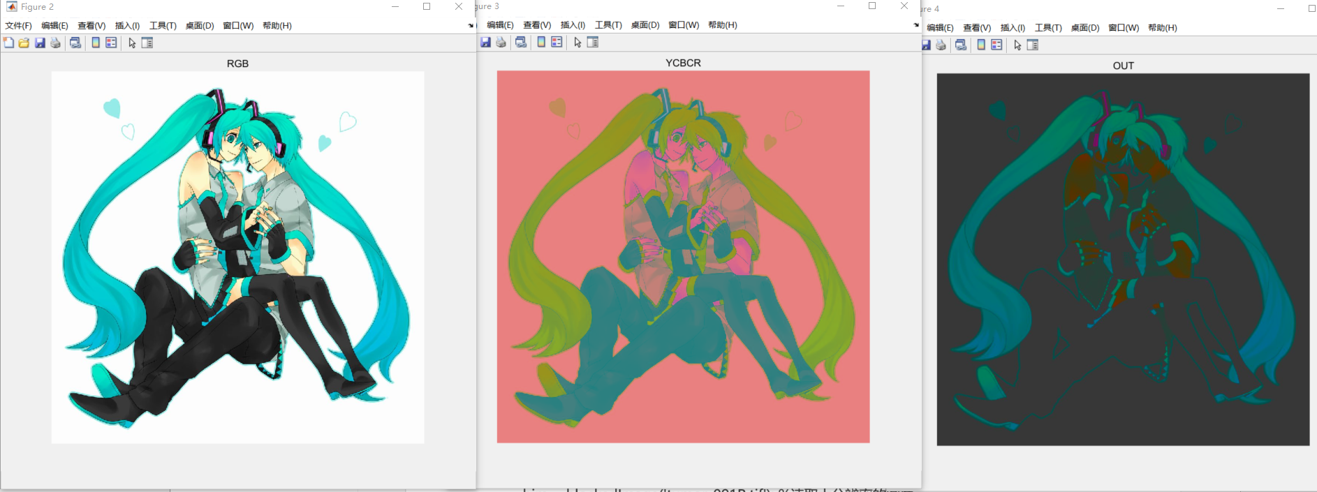
本文算法主要是对图像的亮度调整，故关键点2是颜色空间转换，即要实现对亮度的调整，得把RGB图像转换为YCbCr，然后Y分量即RGB图像的亮度，把算法的结果1000*1000的矩阵的点赋值给Y分量，其他两个分量不变，之后将YCbCr形式的图像转换回RGB图像显示，这时的RGB图像的亮度已经是我们算法的处理结果。关键点1是图像的分块（怎么表示第n块图像块），分块的逆问题：把分块后的图像块组合成一幅图像，通用是利用到主函数里的思路，数字图像即矩阵，即将每个图像块赋值给矩阵的某个范围的行和列即可，如100*100的图像块直接赋值给1000*1000矩阵行和列的1：100范围，把十个图像块循环赋值完，即得到一个矩阵。

 第二组实验图像：

 在上面的图f1中，为经过时间滤波处理后的图像，算法的输出OUT1与原图RGB相比，明显更加明亮鲜艳，整副图像的亮度提升显著，如黑色方框圈出的阳光与原图相比更加耀眼，红色圆圈标注的为暗区域，但算法处理后亮度也有提升，故算法有人工添加的痕迹，整体对比度和亮度改善明显。图g1中，为时间滤波的结果，与f1相比，几乎一致，肉眼很难区别。后面的实验与f1的分析类似，整体亮度和对比度显著增强。

实验结果讨论：

    算法分析，一是从实验看分区100个与1600个，扩大16倍并无明显的视觉改善。二是有无时间滤波，对图像的影响很小。三是，用亮度分量代替RGB进行算法处理，几乎一致。

    若是用到时间滤波，即 公式4，那么首先得计算两帧图像的统计量，即缓存三帧四帧，可以先RGB转换为灰度图像，若是硬件缓存2560*1600@90HZ的RGB视频，若仅仅提取亮度分量Y，一是视频传输带宽为2560*1600*90=368.64MB/S，这仅仅是最小的理论带宽，一般能够满足为千兆网，若是RGB24视频传输带宽，则为1.1GB/S。二是帧缓存，至少两帧用于计算，那么得考虑缓存三帧四帧，缓存大小=2560*1600*4=15.625兆字节。

三 论文算法复现总结

（一）清楚认识世界比你咋想重要得多（首要核心）

       首先得准确理解算法，在算法的设计实现过程中犯了五个误区。

       第一是如算法的处理对象，即LED块的亮度强度，得用颜色空间转换YCbCr才行，而我刚开始直接当成图像的灰度，当成和大多数图像处理算法一样的思路，惯性思维导致。

      第二是，算法是对视频处理，我看到最后才发现这一点，当前帧和上一帧，真的很突然，发现自己想错了，以为搞不来视频仿真，后面才懂直接截取视频两帧图像即可。

      第三是，RGB图像的R分量一开始搞错了，直接写成R =  RGB(1, :, :);% R = 1*M*3. 正确写法如下：R =  RGB(:, :, 1);% R = M*N.

      第四是对于直方图的写法，刚开始直接调用了网上的，后面仔细分析发现统计的灰度值，和直方图代表一个灰度级的像素数差很远。

      第五是，图像的像素总数搞成了图像的灰度总数，这是没有查阅权威资料和文档。这是犯了没有仔细思考，以科学事实为原则。

 （二）循序渐进（拆分原则）

       即设计一个算法，把他拆分成很多步骤或模块组成，例子1如在银行取钱，第一步插入银行卡，第二步输入密码，第三步输入取款金额，第三步取出银行卡离开。例子2，时钟的表针分成三部分，时针，分针，秒针。故本次算法也用拆分，由四个步骤组成，那么就一步步的实现，把第一步实现了做下一步；或者各个击破，把每一步分别实现，组合起来。正确的设计方法，是模块化设计，循序渐进，把每一个部分当成一个函数，直接在主函数调用即可，当遇到问题时，由于是一个模块，且模块间关联不大，很容易解决。很错误就是想一下子把整个功能实现，由于代码量很大，一旦出现问题，会很复杂的逻辑关系，到时候是问题解决你了，败给了时间。

（三）用多种方式去做

     多查阅官方文档，多看权威书籍，多勇敢尝试不同方法，以实践为核心。

 方法1：最开始想复制粘贴别人的算法，发现搜了半天，如CSDN博客，知乎上怎么查找论文的代码列出的网站，博客园，GitHub上，谷歌搜索，搜作者的主页等方式，都没找到，只能另想他法。

方法2：先问了一个同事，他的想法是可以用C++做图像处理，为我开启了一种新思路，但我一直用matlab做红外图像细节增强算法，好歹搞出一篇论文，故不想放弃MATLAB图像处理的基础。他还启发了我，对图像亮度处理，用颜色空间转换: RGB-YCbCr-RGB,让我发现了自己的坑，我设计的算法对图像灰度处理，错的离谱。

方法3：自己编代码。很耗时，同样很多问题伴随，这就是工科生，在问题中收获知识和成长！

了解世界和自己！