三维点云网络PointNet——模型及代码分析

PointNet架构

PointNet主要架构如下图所示：

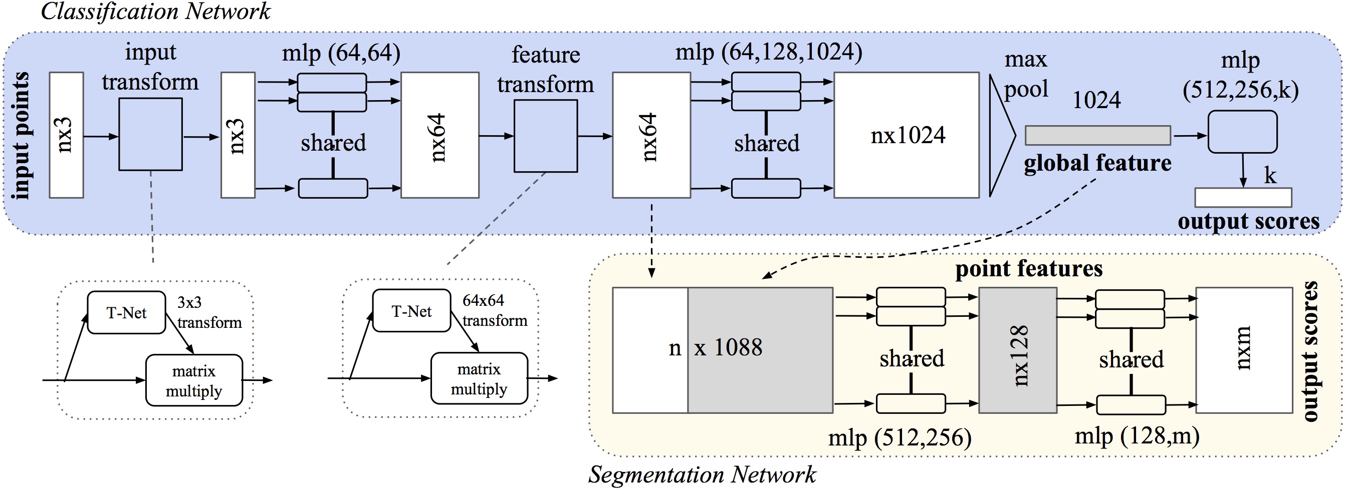
主要包含了点云对齐/转换、mpl学习、最大池化得到全局特征三个主要的部分。

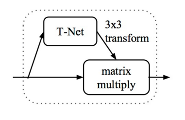
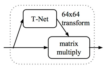
-T-Net用于将不同旋转平移的原始点云和点云特征进行规范化；

• mpl是多层感知机，n个共享的mpl用于处理n个点/特征；
• max pooling 用于融合多个特征并得到全局的1024维的特征；
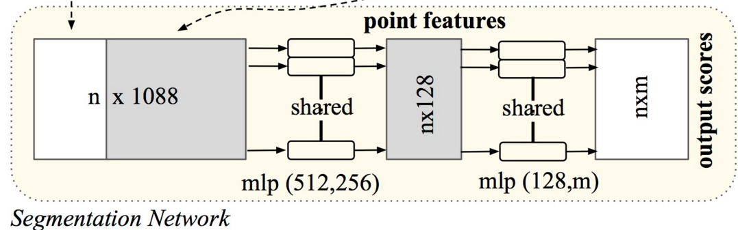
• 最后根据任务的不同，利用一个MPL实现分类；结合局部信息利用多个mpl实现分割。
  

1.T-Net

首先我们来看T-Net模型的代码，它的主要作用是学习出变化矩阵来对输入的点云或特征进行规范化处理。其中包含两个函数，分别是
学习点云变换矩阵的:input_transform_net(point_cloud, is_training, bn_decay=None, K=3)
学习特征变换矩阵的:feature_transform_net(inputs, is_training, bn_decay=None, K=64)

def input_transform_net(point_cloud, is_training, bn_decay=None, K=3):
    """ Input (XYZ) Transform Net, input is BxNx3 gray image
        Return:
            Transformation matrix of size 3xK """
    batch_size = point_cloud.get_shape()[0].value
    num_point = point_cloud.get_shape()[1].value

    input_image = tf.expand_dims(point_cloud, -1)		#转为4D张量
    #构建T-Net模型，64--128--1024
    net = tf_util.conv2d(input_image, 64, [1,3],
                         padding='VALID', stride=[1,1],
                         bn=True, is_training=is_training,
                         scope='tconv1', bn_decay=bn_decay)
    net = tf_util.conv2d(net, 128, [1,1],
                         padding='VALID', stride=[1,1],
                         bn=True, is_training=is_training,
                         scope='tconv2', bn_decay=bn_decay)
    net = tf_util.conv2d(net, 1024, [1,1],
                         padding='VALID', stride=[1,1],
                         bn=True, is_training=is_training,
                         scope='tconv3', bn_decay=bn_decay)
    net = tf_util.max_pool2d(net, [num_point,1],
                             padding='VALID', scope='tmaxpool')

	#利用1024维特征生成256维度的特征
    net = tf.reshape(net, [batch_size, -1])
    net = tf_util.fully_connected(net, 512, bn=True, is_training=is_training,
                                  scope='tfc1', bn_decay=bn_decay)
    net = tf_util.fully_connected(net, 256, bn=True, is_training=is_training,
                                  scope='tfc2', bn_decay=bn_decay)

mpl网络的定义如上，其输入为点云数据，每一个点云作为一个batch。

• 首先将三通道的点云拓展为4-D的张量，tf.expend_dims(),ref,将得到batchn3*1的数据作为网络的输入；
• 随后构建网络，利用1*1的卷积来实现全连接。每一层单元依次为64-128-1024-512-256的网络结构；
  
  接下来需要将mpl得到的256维度特征进行处理，以输出3*3的旋转矩阵：

	#生成点云旋转矩阵 T=3*3
    with tf.variable_scope('transform_XYZ') as sc:
        assert(K==3)
        weights = tf.get_variable('weights', [256, 3*K],
                                  initializer=tf.constant_initializer(0.0),
                                  dtype=tf.float32)
        biases = tf.get_variable('biases', [3*K],
                                 initializer=tf.constant_initializer(0.0),
                                 dtype=tf.float32)
        biases += tf.constant([1,0,0,0,1,0,0,0,1], dtype=tf.float32)
        transform = tf.matmul(net, weights)
        transform = tf.nn.bias_add(transform, biases)

    transform = tf.reshape(transform, [batch_size, 3, K])
    return transform

通过定义权重[W(256,3*K), bais(3*K)]，将上面的256维特征转变为3*3的旋转矩阵输出。

同样对于特征层的规范化处理，其输入为n*64的特征输出为64*64的旋转矩阵，网络结构与上面完全相同，只是在输入输出的维度需要变化：

def feature_transform_net(inputs, is_training, bn_decay=None, K=64):
    """ Feature Transform Net, input is BxNx1xK
        Return:
            Transformation matrix of size KxK """
    batch_size = inputs.get_shape()[0].value
    num_point = inputs.get_shape()[1].value
	
	#构建T-Net模型，64--128--1024
    net = tf_util.conv2d(inputs, 64, [1,1],
                         padding='VALID', stride=[1,1],
                         bn=True, is_training=is_training,
                         scope='tconv1', bn_decay=bn_decay)
    net = tf_util.conv2d(net, 128, [1,1],
                         padding='VALID', stride=[1,1],
                         bn=True, is_training=is_training,
                         scope='tconv2', bn_decay=bn_decay)
    net = tf_util.conv2d(net, 1024, [1,1],
                         padding='VALID', stride=[1,1],
                         bn=True, is_training=is_training,
                         scope='tconv3', bn_decay=bn_decay)
    net = tf_util.max_pool2d(net, [num_point,1],
                             padding='VALID', scope='tmaxpool')

    net = tf.reshape(net, [batch_size, -1])
    net = tf_util.fully_connected(net, 512, bn=True, is_training=is_training,
                                  scope='tfc1', bn_decay=bn_decay)
    net = tf_util.fully_connected(net, 256, bn=True, is_training=is_training,
                                  scope='tfc2', bn_decay=bn_decay)
	
	#生成特征旋转矩阵 T=64*64
    with tf.variable_scope('transform_feat') as sc:
        weights = tf.get_variable('weights', [256, K*K],
                                  initializer=tf.constant_initializer(0.0),
                                  dtype=tf.float32)
        biases = tf.get_variable('biases', [K*K],
                                 initializer=tf.constant_initializer(0.0),
                                 dtype=tf.float32)
        biases += tf.constant(np.eye(K).flatten(), dtype=tf.float32)
        transform = tf.matmul(net, weights)		
        transform = tf.nn.bias_add(transform, biases)

    transform = tf.reshape(transform, [batch_size, K, K])
    return transform

mpl网络定义每一层的神经元数量为64--128--512--256。同样在得到256维的特征后利用weight(256*K*K), bais(K*K)来计算出K*K的特征旋转矩阵，其中K为64,为默认输出特征数量。
代码链接

2.MPL处理点云

在得到点云的规范化选择矩阵后，将原始输入进行处理。旋转后的点云point_cloud_transformed作为MPL的输入抽取特征。

此时输入是旋转后的点云，并通过一个两层的mpl（64--64）得到了64维的特征；

    transform = input_transform_net(point_cloud, is_training, bn_decay, K=3)    # 预测出旋转矩阵T
    point_cloud_transformed = tf.matmul(point_cloud, transform)		  #原始点云乘以旋转矩阵，得到矫正后点云
    input_image = tf.expand_dims(point_cloud_transformed, -1)

	#构建感知机  两层64--64
    net = tf_util.conv2d(input_image, 64, [1,3],
                         padding='VALID', stride=[1,1],
                         bn=True, is_training=is_training,
                         scope='conv1', bn_decay=bn_decay)
    net = tf_util.conv2d(net, 64, [1,1],
                         padding='VALID', stride=[1,1],
                         bn=True, is_training=is_training,
                         scope='conv2', bn_decay=bn_decay)

随后利用特征旋转矩阵transform对特征进行规范化处理，得到校正后的特征。此时的新特征net_transformed将输入到下一个MPL中进行处理

    with tf.variable_scope('transform_net2') as sc:
        transform = feature_transform_net(net, is_training, bn_decay, K=64)    #预测出旋转矩阵T
    end_points['transform'] = transform
    net_transformed = tf.matmul(tf.squeeze(net, axis=[2]), transform)    #特征乘以旋转矩阵，得到矫正后特征
    net_transformed = tf.expand_dims(net_transformed, [2])

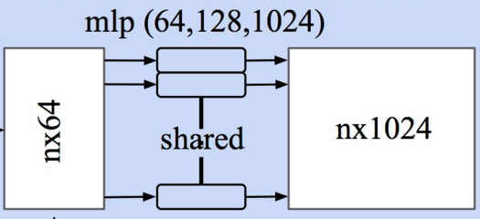
3.MPL处理特征

对于处理点云后的特征需要利用另一个多层感知机进行处理，将表示每个点的输入64维的向量表示为1024维输出：

	#构建mpl 64-128-1024
    net = tf_util.conv2d(net_transformed, 64, [1,1],
                         padding='VALID', stride=[1,1],
                         bn=True, is_training=is_training,
                         scope='conv3', bn_decay=bn_decay)
    net = tf_util.conv2d(net, 128, [1,1],
                         padding='VALID', stride=[1,1],
                         bn=True, is_training=is_training,
                         scope='conv4', bn_decay=bn_decay)
    net = tf_util.conv2d(net, 1024, [1,1],
                         padding='VALID', stride=[1,1],
                         bn=True, is_training=is_training,
                         scope='conv5', bn_decay=bn_decay)

这部分包含三层mpl(64--128--1024),最终输出n*1024维度的特征矩阵.

4.Max Pooling（对称函数）得到全局特征

此时每个输入点从三维变成了1024维的表示，此时需要对n个点所描述的点云进行融合处理以得到全局特征，源码中使用了最大池化层来实现这一功能：

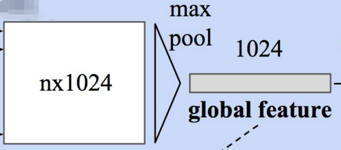
    # Symmetric function: max pooling
    # 最大池化，二维的池化函数对点云中点的数目这个维度进行池化，n-->1
    net = tf_util.max_pool2d(net, [num_point,1],
                             padding='VALID', scope='maxpool')

输出为全局特征[num_point,1]表示将每一个点云的n个点最大池化为1个特征，这个特征的长度为1024。此时通过了两次mpl的处理将一个点云的特征逐点进行描述，并合并到了1024维的全局特征上来。

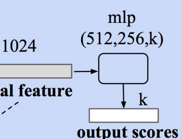
5.分类

利用上面的1024维特征，就可以基于这一特征对点云的特性进行学习实现分类任务，PointNet利用了一个三层感知机MPL(512--256--40)来对特征进行学习，最终实现了对于40类的分类.

    net = tf.reshape(net, [batch_size, -1])

    # 定义分类的mpl512-256-k, k为分类类别数目
    net = tf_util.fully_connected(net, 512, bn=True, is_training=is_training,
                                  scope='fc1', bn_decay=bn_decay)
    net = tf_util.dropout(net, keep_prob=0.7, is_training=is_training,
                          scope='dp1')
    net = tf_util.fully_connected(net, 256, bn=True, is_training=is_training,
                                  scope='fc2', bn_decay=bn_decay)
    net = tf_util.dropout(net, keep_prob=0.7, is_training=is_training,
                          scope='dp2')
    net = tf_util.fully_connected(net, 40, activation_fn=None, scope='fc3')

这一感知机由全连接层组成，其中包含了两个dropout=0.7防止过拟合。最终就可以根据输出K个分类值分数的大小来确定输入点云的分类了。
源码链接

6.分割

对于分割任务，需要加入局域信息来进行学习。所以分类任务的输入包括了1024维的全局信息还包括了n*64的从点云直接学习出的局部信息。PointNet的做法是将全局信息附在每一个局部点描述的后面，形成了1024+64=1088维的向量，而后通过两个感知机来进行分割：

   global_feat_expand = tf.tile(global_feat, [1, num_point, 1, 1])
    concat_feat = tf.concat(3, [point_feat, global_feat_expand])

新得到的特征concat_feat输入两个连续的感知机mpl(512,256),mpl(128,m)都通过1*1卷积实现：

    # 定义分割的mpl512-256-128  128-m, m为点所属的类别数目
    net = tf_util.conv2d(concat_feat, 512, [1,1],
                         padding='VALID', stride=[1,1],
                         bn=True, is_training=is_training,
                         scope='conv6', bn_decay=bn_decay)
    net = tf_util.conv2d(net, 256, [1,1],
                         padding='VALID', stride=[1,1],
                         bn=True, is_training=is_training,
                         scope='conv7', bn_decay=bn_decay)
    net = tf_util.conv2d(net, 128, [1,1],
                         padding='VALID', stride=[1,1],
                         bn=True, is_training=is_training,
                         scope='conv8', bn_decay=bn_decay)
    net = tf_util.conv2d(net, 128, [1,1],
                         padding='VALID', stride=[1,1],
                         bn=True, is_training=is_training,
                         scope='conv9', bn_decay=bn_decay)

    net = tf_util.conv2d(net, 50, [1,1],
                         padding='VALID', stride=[1,1], activation_fn=None,
                         scope='conv10')
    net = tf.squeeze(net, [2]) # BxNxC

由于点云的分割问题可以看做是对于每一个点的分类问题，需要对每一个点的分类进行预测。在通过对全局+局部特征学习后，最后将每一个点分类到50类中，并输出n*50的输出。
代码链接

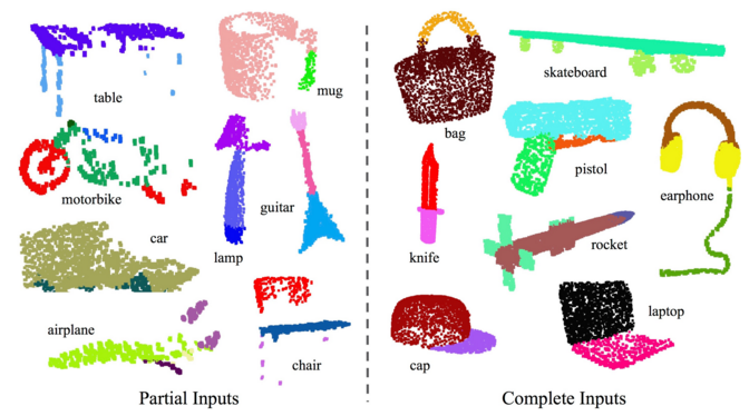
论文中最后的效果如下：

Full code from: https://github.com/charlesq34/pointnet
插图来自pics.sc.chinaz.com