【前言】:之前断断续续看了很多图网络、图卷积网络的讲解和视频。现在对于图网络的理解已经不能单从文字信息中加深了,所以我们要来看代码部分。现在开始看第一篇图网络的论文和代码,来正式进入图网络的科研领域。
- 论文名称:‘GRAPH ATTENTION NETWORKS’
- 文章转自:微信公众号“机器学习炼丹术”
- 笔记作者:炼丹兄
- 联系方式:微信cyx645016617(欢迎交流,共同进步)
- 论文传送门:https://arxiv.org/pdf/1710.10903.pdf
0
1 代码实现
- 代码github:https://github.com/Diego999/pyGAT
- 评价:这个github简洁明了,下载好cora数据集后,直接修改一下路径就可以运行了。我这里的代码讲解也是基于这个github的内容。
1.1 实验结果
因为这是我第一次看GNN的论文,所以我也不知道2018年之后的发展如何(不过估计爆发式发展吧),Graph Attention Network时这样的结果:
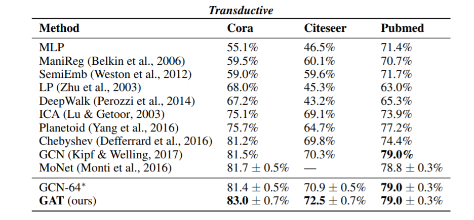
可以看到,cora的精度时0.83左右,而我用官方代码测试的结果为:
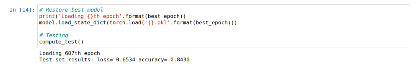
说着至少这是一个比较solid的研究了。
1.2 数据读取
Cora数据集由机器学习论文组成,是近年来图深度学习很喜欢使用的数据集。在数据集中,每一个论文就是一个样本,每一样论文的特征就是某一个单词是否包含在这个论文当中。也就是一个0/1的向量。论文的标签就是论文的类别,总共有7个类别:
- 基于案例
- 遗传算法
- 神经网络
- 概率方法
- 强化学习
- 规则学习
- 理论
论文是一个节点,那么这个节点的邻居有谁那?引用关系。论文的选择方式是,在最终语料库中,每篇论文引用或被至少一篇其他论文引用。整个语料库中有2708篇论文。
在词干堵塞和去除词尾后,只剩下1433个独特的单词。文档频率小于10的所有单词都被删除。
下面是从txt的数据文件中读取,得到每一个样本的标签、特征,以及样本和样本之间的邻接矩阵的函数。
import numpy as np
import scipy.sparse as sp
import torch


def encode_onehot(labels):
    # The classes must be sorted before encoding to enable static class encoding.
    # In other words, make sure the first class always maps to index 0.
    classes = sorted(list(set(labels)))
    classes_dict = {c: np.identity(len(classes))[i, :] for i, c in enumerate(classes)}
    labels_onehot = np.array(list(map(classes_dict.get, labels)), dtype=np.int32)
    return labels_onehot


def load_data(path="./data/cora/", dataset="cora"):
    """Load citation network dataset (cora only for now)"""
    print('Loading {} dataset...'.format(dataset))

    idx_features_labels = np.genfromtxt("{}/{}.content".format(path, dataset), dtype=np.dtype(str))
    features = sp.csr_matrix(idx_features_labels[:, 1:-1], dtype=np.float32)
    labels = encode_onehot(idx_features_labels[:, -1])

    # build graph
    idx = np.array(idx_features_labels[:, 0], dtype=np.int32)
    idx_map = {j: i for i, j in enumerate(idx)}
    edges_unordered = np.genfromtxt("{}/{}.cites".format(path, dataset), dtype=np.int32)
    edges = np.array(list(map(idx_map.get, edges_unordered.flatten())), dtype=np.int32).reshape(edges_unordered.shape)
    adj = sp.coo_matrix((np.ones(edges.shape[0]), (edges[:, 0], edges[:, 1])), shape=(labels.shape[0], labels.shape[0]), dtype=np.float32)

    # build symmetric adjacency matrix
    adj = adj + adj.T.multiply(adj.T > adj) - adj.multiply(adj.T > adj)

    features = normalize_features(features)
    adj = normalize_adj(adj + sp.eye(adj.shape[0]))

    idx_train = range(140)
    idx_val = range(200, 500)
    idx_test = range(500, 1500)

    adj = torch.FloatTensor(np.array(adj.todense()))
    features = torch.FloatTensor(np.array(features.todense()))
    labels = torch.LongTensor(np.where(labels)[1])

    idx_train = torch.LongTensor(idx_train)
    idx_val = torch.LongTensor(idx_val)
    idx_test = torch.LongTensor(idx_test)

    return adj, features, labels, idx_train, idx_val, idx_test


def normalize_adj(mx):
    """Row-normalize sparse matrix"""
    rowsum = np.array(mx.sum(1))
    r_inv_sqrt = np.power(rowsum, -0.5).flatten()
    r_inv_sqrt[np.isinf(r_inv_sqrt)] = 0.
    r_mat_inv_sqrt = sp.diags(r_inv_sqrt)
    return mx.dot(r_mat_inv_sqrt).transpose().dot(r_mat_inv_sqrt)


def normalize_features(mx):
    """Row-normalize sparse matrix"""
    rowsum = np.array(mx.sum(1))
    r_inv = np.power(rowsum, -1).flatten()
    r_inv[np.isinf(r_inv)] = 0.
    r_mat_inv = sp.diags(r_inv)
    mx = r_mat_inv.dot(mx)
    return mx


def accuracy(output, labels):
    preds = output.max(1)[1].type_as(labels)
    correct = preds.eq(labels).double()
    correct = correct.sum()
    return correct / len(labels)
其中,关键的函数就是:
- sp是scipy的sparse库函数,稀疏矩阵操作;
sp.coo_matrix(a,b,c,shape,dtype)这个函数就是构建一个技术矩阵。b是矩阵的行,c是矩阵的列,a是b行c列的那个数字,shape是构建的稀疏矩阵的尺寸。这个函数不清楚可以百度去。这样我们得到的返回值,就是一个矩阵,里面的元素是从被引用文献id指向引用文献的id。adj = adj + adj.T.multiply(adj.T > adj) - adj.multiply(adj.T > adj)
这个方法,就是让有方向的指向变成双向的邻接矩阵。加的第一个因子会重复加上自己引用自己的情况(这种情况再论文中不会出现,但是再其他图网络中可能出现节点连接自己的情况)。而减去的因子就是避免上述重复计算自己连接自己的情况。normalize_feature就是很简单的让每一个样本的特征除以他们的和。使得,每一个样本的特征值的和都是1.normalia_adj类似上面的过程,是让样本的行和列都进行标准化,具体逻辑很难讲清楚,自己体会。
1.3 模型部分
output = model(features, adj)
loss_train = F.nll_loss(output[idx_train], labels[idx_train])
可以看到,模型是把特征和临界矩阵都放进去了,然后输出的output,应该就是每一个样本的分类概率了。之后再通过交叉熵计算得到loss。
model = GAT(nfeat=features.shape[1],
                nhid=8,
                nclass=int(labels.max()) + 1,
                dropout=0.6,
                nheads=8,
                alpha=0.2)
构建GAT的时候,nfeat表示每一个样本的特征数目,这里是1433个,nhid待定含义,nclass就是分类的类别,nheads待定含义,alpha=0.2待定含义。
class GAT(nn.Module):
    def __init__(self, nfeat, nhid, nclass, dropout, alpha, nheads):
        """Dense version of GAT."""
        super(GAT, self).__init__()
        self.dropout = dropout

        self.attentions = [GraphAttentionLayer(nfeat, nhid, dropout=dropout, alpha=alpha, concat=True) for _ in range(nheads)]
        for i, attention in enumerate(self.attentions):
            self.add_module('attention_{}'.format(i), attention)

        self.out_att = GraphAttentionLayer(nhid * nheads, nclass, dropout=dropout, alpha=alpha, concat=False)

    def forward(self, x, adj):
        x = F.dropout(x, self.dropout, training=self.training)
        x = torch.cat([att(x, adj) for att in self.attentions], dim=1)
        x = F.dropout(x, self.dropout, training=self.training)
        x = F.elu(self.out_att(x, adj))
        return F.log_softmax(x, dim=1)
上面就是模型构建的pytorch模型类。可以发现:
- 有几个nhead,self.attentions中就会有几个GraphAttentionLayer。最后再加一个
self.out_att的GraphAttentionLayer,就构成了全部的网络。 - forward阶段,特征先进行随机的dropout,dropout率这么大不知道是不是图网络都是这样的,六个悬念把。
- 经过dropout的模型,分别经过之前不同的nheads定义的GraphAttentionLayer,然后把所有的结果都concat起来;
- 再进行一次dropout后,就进行
sefl.out_att就行了。最后用softmax一下就好。
现在其中的关键就是GraphAttentionLayer的构建了
1.4 GraphAttentionLayer
class GraphAttentionLayer(nn.Module):
    """
    Simple GAT layer, similar to https://arxiv.org/abs/1710.10903
    """
    def __init__(self, in_features, out_features, dropout, alpha, concat=True):
        super(GraphAttentionLayer, self).__init__()
        self.dropout = dropout
        self.in_features = in_features
        self.out_features = out_features
        self.alpha = alpha
        self.concat = concat

        self.W = nn.Parameter(torch.empty(size=(in_features, out_features)))
        nn.init.xavier_uniform_(self.W.data, gain=1.414)
        self.a = nn.Parameter(torch.empty(size=(2*out_features, 1)))
        nn.init.xavier_uniform_(self.a.data, gain=1.414)

        self.leakyrelu = nn.LeakyReLU(self.alpha)

    def forward(self, h, adj):
        Wh = torch.mm(h, self.W) # h.shape: (N, in_features), Wh.shape: (N, out_features)
        e = self._prepare_attentional_mechanism_input(Wh)

        zero_vec = -9e15*torch.ones_like(e)
        attention = torch.where(adj > 0, e, zero_vec)
        attention = F.softmax(attention, dim=1)
        attention = F.dropout(attention, self.dropout, training=self.training)
        h_prime = torch.matmul(attention, Wh)

        if self.concat:
            return F.elu(h_prime)
        else:
            return h_prime

    def _prepare_attentional_mechanism_input(self, Wh):
        # Wh.shape (N, out_feature)
        # self.a.shape (2 * out_feature, 1)
        # Wh1&2.shape (N, 1)
        # e.shape (N, N)
        Wh1 = torch.matmul(Wh, self.a[:self.out_features, :])
        Wh2 = torch.matmul(Wh, self.a[self.out_features:, :])
        # broadcast add
        e = Wh1 + Wh2.T
        return self.leakyrelu(e)

    def __repr__(self):
        return self.__class__.__name__ + ' (' + str(self.in_features) + ' -> ' + str(self.out_features) + ')'
这个GraphAttentionLayer(GAL)中的forward函数,h就是features,shape应该是(2708,1433),adj是节点的邻接矩阵,shape是(2708,2708)
- 先用h通过torch.mm得到隐含变量,类似于一个全连接层,把1433个特征缩小到8个特征(nhid=8);
e = self._prepare_attentional_mechanism_input(Wh)这一段应该是这篇论文创新的地方了。这一段里面实在是太抽象了,要看论文才能理解它的含义把可坑,反正这个函数返回的e的shape是(2708,2708)torch.where这是一个新的函数。在使用A[A>x] = 1这样的in-place操作是不可导的,所以我要使用torch.where(condiciton,B,A)函数。满足条件的A会被对应位置的B替代。所以代码中就是,zero_vec的邻接矩阵大于0的位置的值会被替换成刚刚计算出来的e的对应位置的值。这个就是atteniton,表示临界的节点对于这个节点的不同的重要性的概念把。然后就是dropout,然后就是attention和W相乘。结束了。
【总结一下】,首先经过全连接层讲1433特征压缩成8个特征,然后通过某种机制得到一个注意力权重,然后根据邻接矩阵选出来一部分的权重值,然后在一开始的8个特征进行相乘即可。
1.5 疑惑
这一行代码:
# init部分
self.attentions = [GraphAttentionLayer(nfeat, nhid, dropout=dropout, alpha=alpha, concat=True) for _ in range(nheads)]
# forward部分
x = torch.cat([att(x, adj) for att in self.attentions], dim=1)
为什么要构建8个一摸一样的GraphAttentionLayer呢?我感觉就是你用8个一摸一样的卷积层并列起来,其实并不能起到增强特征的效果。
所以我这里使用了不同的nheads来进行实验,看看是否对实验结果有影响:
| nheads | test acc |
|---|---|
| 8 | 0.84 |
| 4 | 0.848 |
| 2 | 0.841 |
| 1 | 0.8450 |
| 12 | 0.8480 |
实验结果表明,其实nheads的个数,对实际的影响并不大,不过既然都做到这里了,我们再来看一下nhid对于实验结果的影响,这里选择nheads为1
| nhid | test acc |
|---|---|
| 8 | 0.84 |
| 16 | 0.8500 |
| 32 | 0.8400 |
| 64 | 0.8350 |
| 4 | 0.7940 |
实验结果表明,nhid太少造成特征缺失,太多又容易过拟合。所以要选择始中才好