python - 3.7
pycharm
numpy-1.15.1
pandas-0.23.4
matplotlib-2.2.3
"""
    梯度计算:对J(θ)求θ的偏导
"""


def gradient(X, Y, theta):
    grad = np.zeros(theta.shape)  # 根据3个不同的θ求出对应的梯度
    error = (model(X, theta) - Y).ravel()  # 将J(θ)偏导xij之前的那一部分提出来
    for j in range(len(theta.ravel())):  # θ0~θ2,
        term = np.multiply(error, X[:, j])  # 这里计算的不是单个数值,而是一列的数值,每一步需要计算每个样的的θ0,下一次计算每一个样本的θ1...
        grad[0, j] = np.sum(term) / len(X)  # 填充每一个θ的梯度,[1,3]的结构
    return grad


"""
    比较3种不同梯度下降的方法
    批量,随机,小批量

"""

"""
    三种停止方法
"""
STOP_ITER = 0  # 迭代次数
STOP_COST = 1  # 损失值,差异非常小
STOP_GRAD = 2  # 梯度,梯度变化非常小


def stopCriterion(type, value, threshold):  # type=停止方式,value=实际值,threshold=阈值
    if type == STOP_ITER:
        return value > threshold  # 此处value是迭代次数
    elif type == STOP_COST:
        return abs(value[-1] - value[-2]) < threshold  # 此处value是损失值,用最后一个损失值减去倒数第二个损失值,看看是否小于阈值
    elif type == STOP_GRAD:
        return np.linalg.norm(value) < threshold  # 此处value是梯度,求矩阵的范数,看看是否收敛


"""
    洗牌,打乱数据顺序
"""


def shuffleData(data):
    np.random.shuffle(data)
    cols = data.shape[1]
    X = data[:, 0:cols - 1]  # 洗牌后取X
    Y = data[:, cols - 1:]  # 洗牌后取Y
    return X, Y


"""
    看时间的影响
"""

import time


def descent(data, theta, batchSize, stopType, thresh,
            alpha):  # data=数据,theta=θ,batchSize=样本数,stopType=停止策略,thresh=阈值,alpha=学习率
    # 梯度下降求解
    init_time = time.time()
    i = 0  # 迭代次数
    k = 0  # batch
    X, Y = shuffleData(data)
    grad = np.zeros(theta.shape)  # 计算的梯度
    costs = [cost(X, Y, theta)]  # 损失值

    while True:
        grad = gradient(X[k:k + batchSize], Y[k:k + batchSize], theta)
        k = k + batchSize
        if k >= n:  # 样本数
            k = 0
            X, Y = shuffleData(data)  # 洗牌
        theta = theta - alpha * grad  # 参数更新
        costs.append(cost(X, Y, theta))  # 计算新的损失值,要画图,所以要每一次的损失值
        i = i + 1

        if stopType == STOP_ITER:
            value = i
        elif stopType == STOP_COST:
            value = costs
        elif stopType == STOP_GRAD:
            value = grad
        if stopCriterion(stopType, value, thresh):
            break
    return theta, i - 1, costs, grad, time.time() - init_time


def runExpe(data, theta, batchSize, stopType, thresh, alpha):
    theta, iter, costs, grad, dur = descent(data, theta, batchSize, stopType, thresh, alpha)  # dur是用时
    name = 'Original' if (data[:, 1] > 2).sum() > 1 else 'Scaled'
    name += 'data- learning rate:{}-'.format(alpha)
    if batchSize == n:
        strDescType = 'Gradient'
    elif batchSize == 1:
        strDescType = 'Stochastic'
    else:
        strDescType = 'Mini-Batch({})'.format(batchSize)

    name += strDescType + 'descentStop:'
    if stopType == STOP_ITER:
        strStop = "{}-iterations".format(thresh)
    elif stopType == STOP_COST:
        strStop = "cost change <{}".format(thresh)
    else:
        strStop = 'gradient norm<{}'.format(thresh)
    name += strStop
    print("***{}
Theta:{}-Iter:{}-Last cost:{:03.2f}-Duration:{:03.2f}s".format(name, theta, iter, costs[-1], dur))
    fig, ax = plt.subplots(figsize = (12, 4))
    ax.plot(np.arange(len(costs)), costs, 'r')
    ax.set_xlabel('Iterations')
    ax.set_ylabel('Cost')
    ax.set_title(name.upper() + "Error vs.Iteration")
    plt.show()
    return theta


"""
    不同停止策略
"""
"""
    设定迭代次数
"""
# 选择梯度下降的方法是基于所有样本的
n = 100  # 样本数100
runExpe(orig_data, theta, n, STOP_ITER, thresh = 5000, alpha = 0.000001)  # 迭代次数5000次,
运行结果:
***Originaldata- learning rate:1e-06-GradientdescentStop:5000-iterations
Theta:[[-0.00027127 0.00705232 0.00376711]]-Iter:5000-Last cost:0.63-Duration:1.22s
Process finished with exit code 0
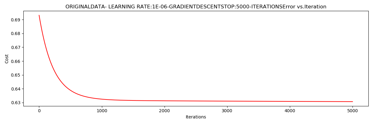
整体梯度下降,策略是迭代次数,学习率非常小,看似收敛于0.63,用时1.18秒,非常快。
"""
    根据损失值停止
"""
n = 100
runExpe(orig_data, theta, n, STOP_COST, thresh = 0.000001, alpha = 0.001)
运行结果:
***Originaldata- learning rate:0.001-GradientdescentStop:cost change <1e-06
Theta:[[-5.13364014 0.04771429 0.04072397]]-Iter:109901-Last cost:0.38-Duration:26.95s
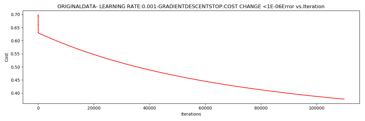
根据损失值停止,使得
$Jleft ( Theta_{last} ight )-Jleft ( Theta_{last-1} ight )$<0.000001,
迭代次数达到了110000次
$Jleft ( Theta ight )$收敛于0.38
迭代次数为109901,
用时:26.95s
"""
    根据梯度下降值停止
"""
n = 100
runExpe(orig_data, theta, n, STOP_GRAD, thresh = 0.05, alpha = 0.001)
运行结果:
***Originaldata- learning rate:0.001-GradientdescentStop:gradient norm<0.05
Theta:[[-2.37033409 0.02721692 0.01899456]]-Iter:40045-Last cost:0.49-Duration:9.79s
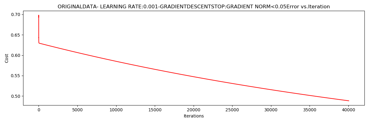
梯度下降
梯度矩阵的范数小于0.05,
$Jleft ( Theta ight )$
收敛于0.49
迭代次数为40045,
用时:9.79s
"""
不同梯度下降方法
"""
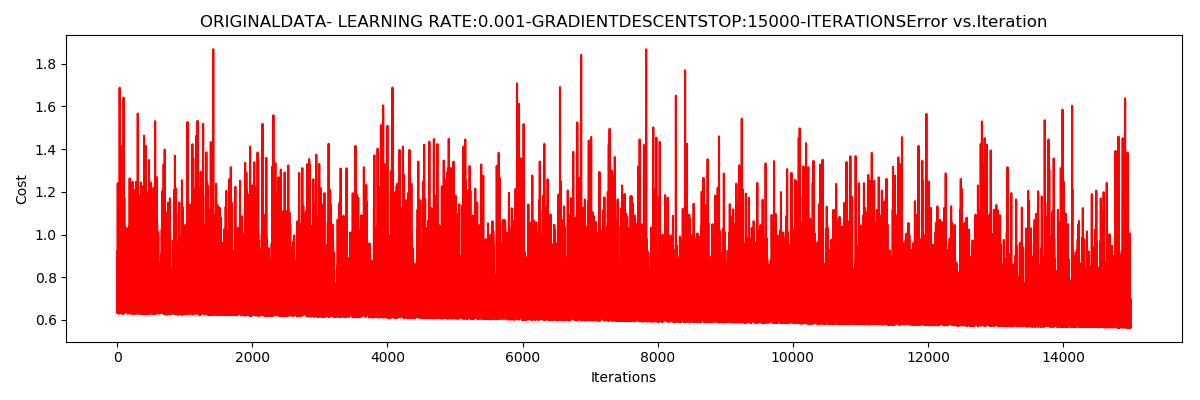
# 随机样本
n = 1
runExpe(orig_data, theta, n, STOP_ITER, thresh = 5000, alpha = 0.001)
运行结果:
***Originaldata- learning rate:0.001-GradientdescentStop:5000-iterations
Theta:[[-0.37366988 -0.06178623 -0.00857957]]-Iter:5000-Last cost:3.39-Duration:1.20s

随机样本个数
迭代次数5000,
样本数为1
不收敛
迭代次数为5000,
用时:1.20s
当把学习率调小一些:
# 随机样本-调小学习率
n = 1
runExpe(orig_data, theta, n, STOP_ITER, thresh = 15000, alpha = 0.000002)
运行结果:
***Originaldata- learning rate:2e-06-GradientdescentStop:15000-iterations
Theta:[[-0.00201849 0.01062308 0.0019506 ]]-Iter:15000-Last cost:0.63-Duration:3.62s
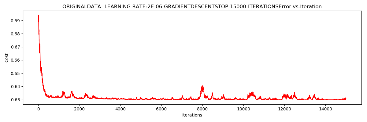
随机样本个数
迭代次数15000,
学习率0.000002
$Jleft ( Theta ight )$
收敛于0.63
迭代次数为15000,
用时:3.62s
结果也不是很好
# 小批量样本
n = 16
runExpe(orig_data, theta, n, STOP_ITER, thresh = 15000, alpha = 0.001)
运行结果:
***Originaldata- learning rate:0.001-GradientdescentStop:15000-iterations
Theta:[[-1.01943681e+00 1.48973461e-02 8.16026410e-04]]-Iter:15000-Last cost:0.62-Duration:3.54s
小批量样本个数
迭代次数15000,
学习率0.001
$Jleft ( Theta ight )$
不收敛
迭代次数为15000,
用时:3.54s
"""
    数据标准化:
        将其数据按列减去均值,然后除以方差,最后得到的结果是,对每个属性(按列)
        所有数据的均值都是0,方差为1
"""
from sklearn import preprocessing as pp
n = 1
scaled_data = orig_data.copy()
scaled_data[:, 1:3] = pp.scale(orig_data[:, 1:3])
runExpe(scaled_data, theta, n, STOP_ITER, thresh = 5000, alpha = 0.001)
运行结果:
***Scaleddata- learning rate:0.001-GradientdescentStop:5000-iterations
Theta:[[0.31719248 0.87056109 0.7704687 ]]-Iter:5000-Last cost:0.38-Duration:1.18s
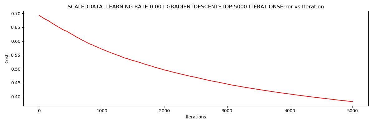
经过数据初始化之后的随机样本个数
迭代次数5000,
样本数为1
$Jleft ( Theta ight )$
收敛于0.38
迭代次数为5000,
用时:1.18s
# 批量梯度下降
n = 100
runExpe(scaled_data, theta, n, STOP_GRAD, thresh = 0.02, alpha = 0.001)
运行结果:
***Scaleddata- learning rate:0.001-GradientdescentStop:gradient norm<0.02
Theta:[[1.0707921 2.63030842 2.41079787]]-Iter:59422-Last cost:0.22-Duration:15.70s
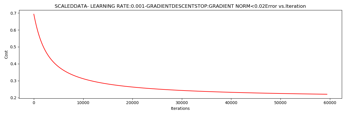
批量梯度下降
迭代次数59422,
样本数为100
梯度范数阈值:0.02”
$Jleft ( Theta ight )$
收敛于0.22
用时:15.70s
# 小批量梯度下降
n = 16
runExpe(scaled_data, theta, n, STOP_GRAD, thresh = 0.02*2, alpha = 0.001)
运行结果:
***Scaleddata- learning rate:0.001-GradientdescentStop:gradient norm<0.004
Theta:[[1.13294 2.75139821 2.53118872]]-Iter:69258-Last cost:0.22-Duration:18.31s
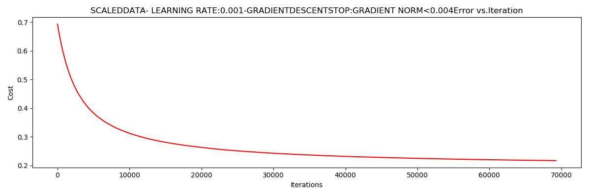
小批量梯度下降
迭代次数69258,
样本数为16
梯度范数阈值:0.002*2
$Jleft ( Theta ight )$
收敛于0.22
用时:18.31s
"""
    精度
"""


# 设定阈值
def predict(X, theta):  # 分类函数
    return [1 if x >= 0.5 else 0 for x in model(X, theta)]  # 概率大于0.5能被录取,概率小鱼0.5则不能被录取


scaled_X = scaled_data[:, :3]
Y = scaled_data[:, 3]
predictions = predict(scaled_X, theta)
correct = [1 if ((a == 1 and b == 1) or (a == 0 and b == 0)) else 0 for a, b in zip(predictions, Y)]  # 看看有多少和原数据预测一致
accuracy = (sum(map(int, correct)) % len(correct))
print('accurent ={0}%'.format(accuracy))
运行结果:
accurent =60%
视频中为什么是89%
同样的数据同样的代码,差别为什么会这么大?
步骤总结:
1,先在数据中添加一列
2,按照每个函数流程
    `sigmoid` : 映射到概率的函数
    `model` : 返回预测结果值
    `cost` : 根据参数计算损失
    `gradient` : 计算每个参数的梯度方向
    `descent` : 进行参数更新
    `accuracy`: 计算精度