TensorFlow 手写体数字识别

TensorFlow 手写体数字识别

  以下资料来源于极客时间学习资料

• 手写体数字 MNIST 数据集介绍

MNIST 数据集介绍

 

　　MNIST 是一套手写体数字的图像数据集，包含 60,000 个训练样例和 10,000 个测试样例，

由纽约大学的 Yann LeCun 等人维护。

 

获取 MNIST 数据集

 

MNIST 手写体数字介绍

 

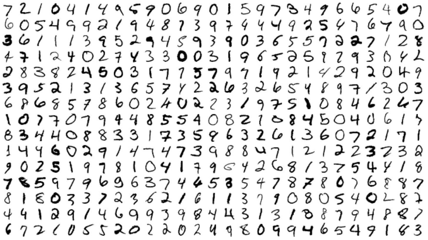
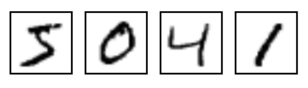
　　MNIST 图像数据集使用形如［28，28］的二阶数组来表示每个手写体数字，数组中

的每个元素对应一个像素点，即每张图像大小固定为 28x28 像素。

　　MNIST 数据集中的图像都是256阶灰度图，即灰度值 0 表示白色（背景），255 表示

黑色（前景），使用取值为［0，255］的uint8数据类型表示图像。为了加速训练，我

们需要做数据规范化，将灰度值缩放为［0，1］的float32数据类型。

 

 

下载和读取 MNIST 数据集

 

　　一个曾广泛使用（如 chapter-2/basic-model.ipynb），如今被废弃的（deprecated）方法：

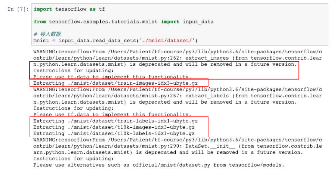
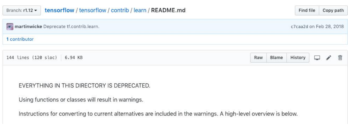
tf.contrib.learn 模块已被废弃

　　需要注意的是，tf.contrib.learn 整个模块均已被废弃：

 

 

使用 Keras 加载 MNIST 数据集

tf.kera.datasets.mnist.load_data(path=‘mnist.npz’)

Arguments:

• path:本地缓存 MNIST 数据集(mnist.npz)的相对路径（~/.keras/datasets）

Returns：

　　Tuple of Numpy arrays: `(x_train, y_train), (x_test, y_test)`.

 

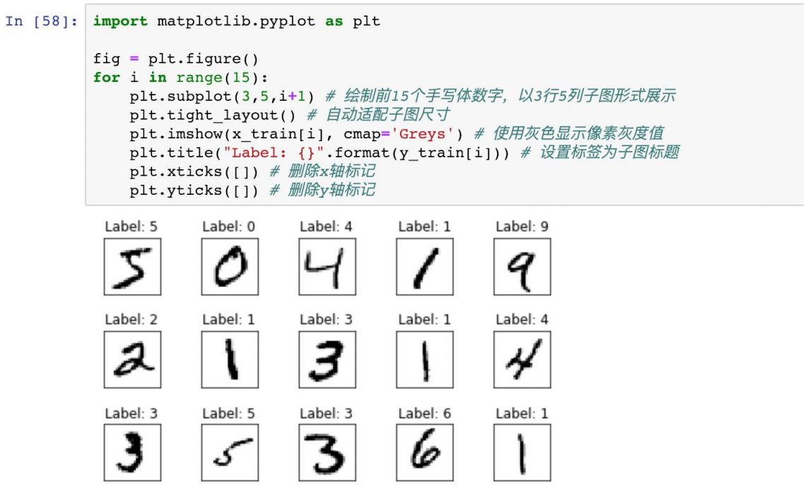
MNIST 数据集 样例可视化

 

• MNIST Softmax 网络介绍

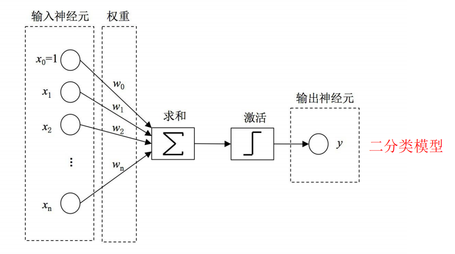
感知机模型

 

　　1957年，受 Warren McCulloch 和 Walter Pitts 在神经元建模方面工作的启发，心理学家 Frank

Rosenblatt 参考大脑中神经元信息传递信号的工作机制，发明了神经感知机模型 Perceptron 。 

 

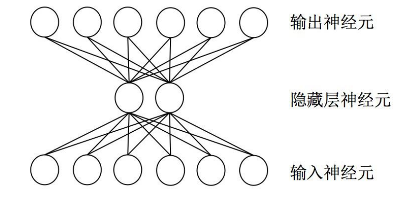
神经网络 

 

　　在机器学习和认知科学领域，人工神经网络（ANN），简称神经网络（NN）是一种模仿生物

神经网络（动物的中枢神经系统，特别是大脑）的结构和功能的数学模型或计算模型，用于

对函数进行估计或近似。神经网络是多层神经元的连接，上一层神经元的输出，作为下一层

神经元的输入。

 

线性不可分

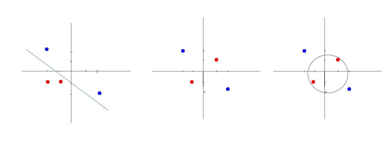
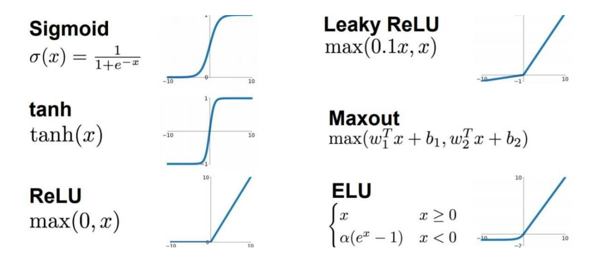
激活函数（Activation Function） 

 

　　为了实现神经网络的非线性建模能力，解决一些线性不可分的问题，我们通常使用激活函数

来引入非线性因素。激活函数都采用非线性函数，常用的有Sigmoid、tanh、ReLU等。

 

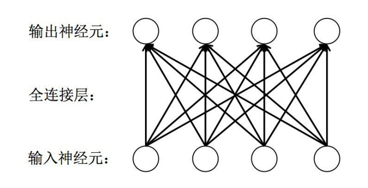
全连接层（ fully connected layers，FC ）

 

　　全连接层是一种对输入数据直接做线性变换的线性计算层。它是神经网络中最常用的一种层，

用于学习输出数据和输入数据之间的变换关系。全连接层可作为特征提取层使用，在学习特

征的同时实现特征融合；也可作为最终的分类层使用，其输出神经元的值代表了每个输出类

别的概率。

 

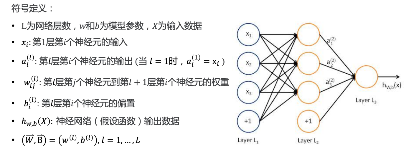
前向传播

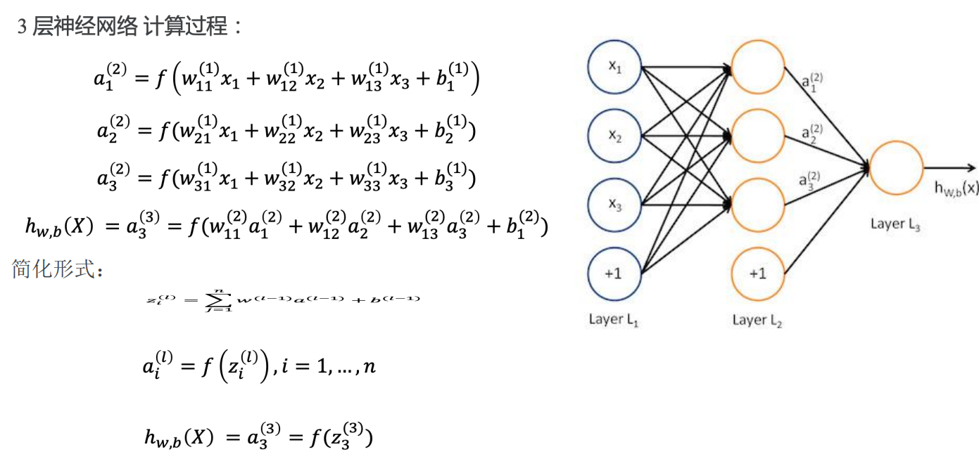
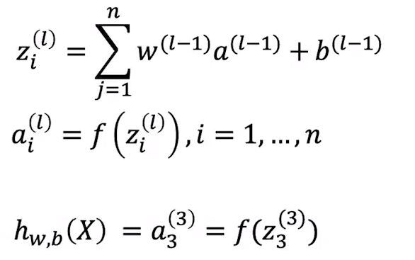
 简化形式：

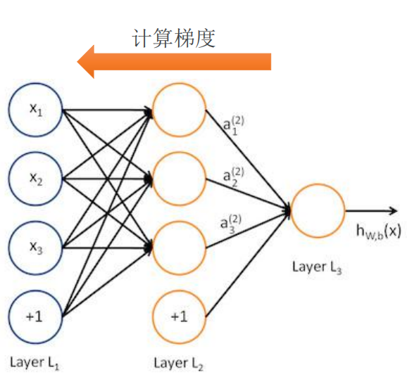
后向传播（ Back Propagation, BP） 

 

　　BP算法的基本思想是通过损失函数对模型参数进行求导，并根据复合函数求导常用的 “链式法则” 将不同层的模型参

数的梯度联系起来，使得计算所有模型参数的梯度更简单。BP算法的思想早在 1960s 就被提出来了。 直到1986年，

David Rumelhart 和 Geoffrey Hinton 等人发表了一篇后来成为经典的论文，清晰地描述了BP算法的框架，才使得BP算

法真正流行起来，并带来了神经网络在80年代的辉煌。 

 

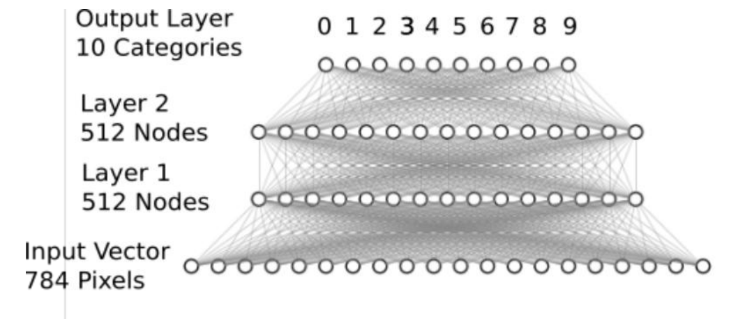
MNIST Softmax 网络 

 

　　将表示手写体数字的形如 [784] 的一维向量作为输入；中间定义2层 512 个神经元的隐藏层，具

备一定模型复杂度，足以识别手写体数字；最后定义1层10个神经元的全联接层，用于输出10

个不同类别的“概率”。

Softmax :

　　在数学，尤其是概率论和相关领域中，Softmax函数，或称归一化指数函数，是逻辑函数的一种推广。

Softmax函数实际上是有限项离散概率分布的梯度对数归一化。

 

• 实战 MNIST Softmax 网络

MNIST Softmax 网络层

代码： 

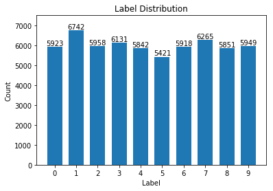
加载 MNIST 数据集    
from keras.datasets import mnist

(x_train, y_train), (x_test, y_test) = mnist.load_data('mnist/mnist.npz')

print(x_train.shape, type(x_train))
print(y_train.shape, type(y_train))
'''
(60000, 28, 28) <class 'numpy.ndarray'>
(60000,) <class 'numpy.ndarray'>
'''

数据处理：规范化
# 将图像本身从[28,28]转换为[784,]
X_train = x_train.reshape(60000, 784)
X_test = x_test.reshape(10000, 784)
print(X_train.shape, type(X_train))
print(X_test.shape, type(X_test))
'''
(60000, 784) <class 'numpy.ndarray'>
(10000, 784) <class 'numpy.ndarray'>
'''

# 将数据类型转换为float32
X_train = X_train.astype('float32')
X_test = X_test.astype('float32')
# 数据归一化
X_train /= 255
X_test /= 255

统计训练数据中各标签数量
import numpy as np
import matplotlib.pyplot as plt

label, count = np.unique(y_train, return_counts=True)
print(label, count)
'''
[0 1 2 3 4 5 6 7 8 9] [5923 6742 5958 6131 5842 5421 5918 6265 5851 5949]
'''

fig = plt.figure()
plt.bar(label, count, width = 0.7, align='center')
plt.title("Label Distribution")
plt.xlabel("Label")
plt.ylabel("Count")
plt.xticks(label)
plt.ylim(0,7500)

for a,b in zip(label, count):
    plt.text(a, b, '%d' % b, ha='center', va='bottom',fontsize=10)

plt.show()

数据处理：one-hot 编码

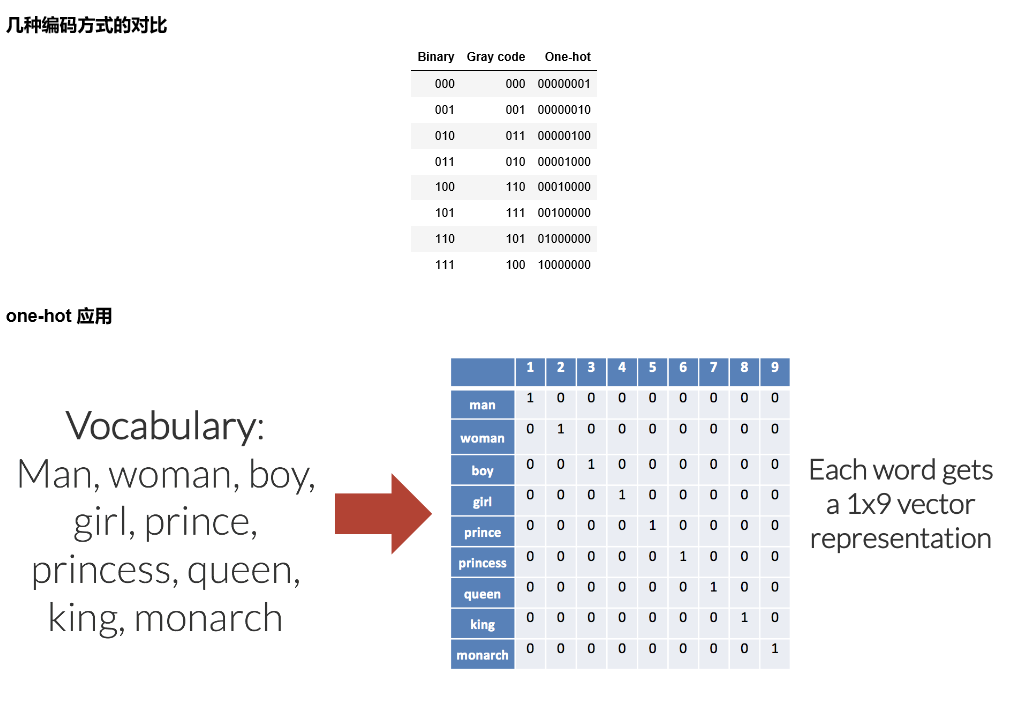
from keras.utils import np_utils

n_classes = 10
print("Shape before one-hot encoding: ", y_train.shape)
Y_train = np_utils.to_categorical(y_train, n_classes)
print("Shape after one-hot encoding: ", Y_train.shape)
Y_test = np_utils.to_categorical(y_test, n_classes)
'''
Shape before one-hot encoding:  (60000,)
Shape after one-hot encoding:  (60000, 10)
'''

print(y_train[0])
print(Y_train[0])
'''
5
[0. 0. 0. 0. 0. 1. 0. 0. 0. 0.]
'''

使用 Keras sequential model 定义神经网络
softmax 网络层

from keras.models import Sequential
from keras.layers.core import Dense, Activation

model = Sequential()
model.add(Dense(512, input_shape=(784,)))
model.add(Activation('relu'))                            

model.add(Dense(512))
model.add(Activation('relu'))

model.add(Dense(10))
model.add(Activation('softmax'))

编译模型

model.compile(loss='categorical_crossentropy', metrics=['accuracy'], optimizer='adam')


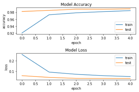
训练模型，并将指标保存到 history 中

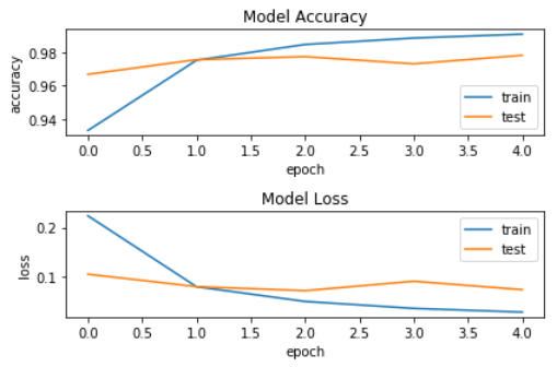
history = model.fit(X_train,
                    Y_train,
                    batch_size=128,
                    epochs=5,
                    verbose=2,
                    validation_data=(X_test, Y_test))
'''


Train on 60000 samples, validate on 10000 samples
Epoch 1/5
 - 5s - loss: 0.2240 - acc: 0.9331 - val_loss: 0.1050 - val_acc: 0.9668
Epoch 2/5
 - 5s - loss: 0.0794 - acc: 0.9753 - val_loss: 0.0796 - val_acc: 0.9756
Epoch 3/5
 - 5s - loss: 0.0494 - acc: 0.9847 - val_loss: 0.0714 - val_acc: 0.9774
Epoch 4/5
 - 6s - loss: 0.0353 - acc: 0.9886 - val_loss: 0.0906 - val_acc: 0.9731
Epoch 5/5
 - 6s - loss: 0.0277 - acc: 0.9909 - val_loss: 0.0735 - val_acc: 0.9782
'''

可视化指标
fig = plt.figure()
plt.subplot(2,1,1)
plt.plot(history.history['acc'])
plt.plot(history.history['val_acc'])
plt.title('Model Accuracy')
plt.ylabel('accuracy')
plt.xlabel('epoch')
plt.legend(['train', 'test'], loc='lower right')

plt.subplot(2,1,2)
plt.plot(history.history['loss'])
plt.plot(history.history['val_loss'])
plt.title('Model Loss')
plt.ylabel('loss')
plt.xlabel('epoch')
plt.legend(['train', 'test'], loc='upper right')
plt.tight_layout()

plt.show()

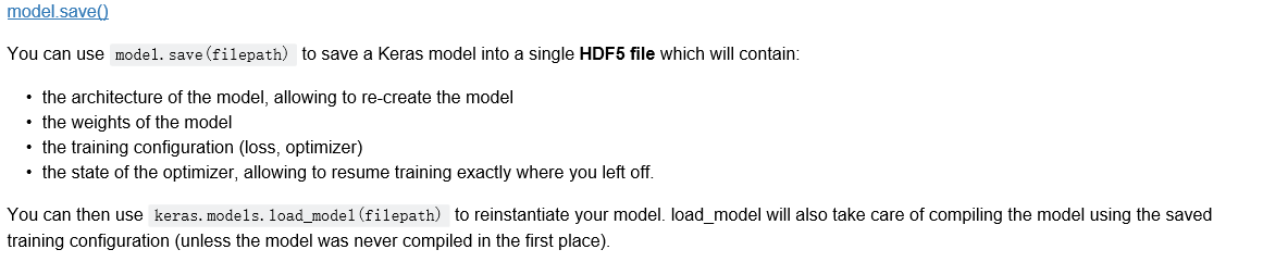
保存模型

import os
import tensorflow.gfile as gfile

save_dir = "./mnist/model/"

if gfile.Exists(save_dir):
    gfile.DeleteRecursively(save_dir)
gfile.MakeDirs(save_dir)

model_name = 'keras_mnist.h5'
model_path = os.path.join(save_dir, model_name)
model.save(model_path)
print('Saved trained model at %s ' % model_path)
'''
Saved trained model at ./mnist/model/keras_mnist.h5 
'''

加载模型
from keras.models import load_model

mnist_model = load_model(model_path)

统计模型在测试集上的分类结果
loss_and_metrics = mnist_model.evaluate(X_test, Y_test, verbose=2)
    
print("Test Loss: {}".format(loss_and_metrics[0]))
print("Test Accuracy: {}%".format(loss_and_metrics[1]*100))

predicted_classes = mnist_model.predict_classes(X_test)

correct_indices = np.nonzero(predicted_classes == y_test)[0]
incorrect_indices = np.nonzero(predicted_classes != y_test)[0]
print("Classified correctly count: {}".format(len(correct_indices)))
print("Classified incorrectly count: {}".format(len(incorrect_indices)))
'''
Test Loss: 0.07348056956584333
Test Accuracy: 97.82%
Classified correctly count: 9782
Classified incorrectly count: 218
'''

• MNIST CNN 网络介绍

CNN 简介

 

　　CNN模型是一种以卷积为核心的前馈神经网络模型。 20世纪60年代，Hubel和Wiesel在研究猫脑

皮层中用于局部敏感和方向选择的神经元时发现其独特的网络结构可以有效地降低反馈神经网

络的复杂性，继而提出了卷积神经网络（ConvoluTIonal Neural Networks，简称CNN）。

 

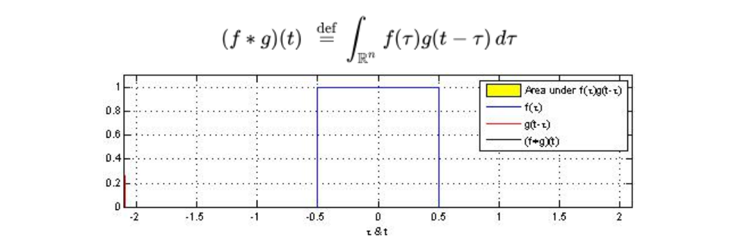
卷积（Convolution）

 

　　卷积是分析数学中的一种基础运算，其中对输入数据做运算时所用到的函数称为卷积核。

设:f(x), g(x)是R上的两个可积函数，作积分： 

 

　　可以证明，关于几乎所有的实数x，上述积分是存在的。这样，随着x的不同取值，这个积分就

定义了一个如下的新函数，称为函数f与g的卷积

 

卷积层（Convolutional Layer, conv） 

 

　　卷积层是使用一系列卷积核与多通道输入数据做卷积的线性计算层。卷积层的提出是为了利用

输入数据（如图像）中特征的局域性和位置无关性来降低整个模型的参数量。卷积运算过程与

图像处理算法中常用的空间滤波是类似的。因此，卷积常常被通俗地理解为一种“滤波”过程，

卷积核与输入数据作用之后得到了“滤波”后的图像，从而提取出了图像的特征。

 

池化层（Pooling） 

 

　　池化层是用于缩小数据规模的一种非线性计算层。为了降低特征维度，我们需要对输入数据进

行采样，具体做法是在一个或者多个卷积层后增加一个池化层。池化层由三个参数决定：（1）

池化类型，一般有最大池化和平均池化两种；（2）池化核的大小k；（3）池化核的滑动间隔s。

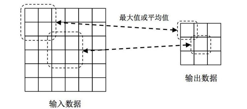
下图给出了一种的池化层示例。其中，2x2大小的池化窗口以2个单位距离在输入数据上滑动。

在池化层中，如果采用最大池化类型，则输出为输入窗口内四个值的最大值；如采用平均池化

类型，则输出为输入窗口内四个值的平均值

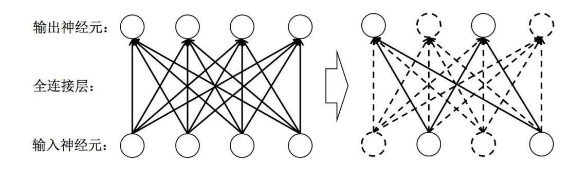
Dropout 层 

 

　　Dropout 是常用的一种正则化方法，Dropout层是一种正则化层。全连接层参数量非常庞大（占

据了CNN模型参数量的80%～90%左右），发生过拟合问题的风险比较高，所以我们通常需要

一些正则化方法训练带有全连接层的CNN模型。在每次迭代训练时，将神经元以一定的概率值

暂时随机丢弃，即在当前迭代中不参与训练。

Flatten 

 

　　将卷积和池化后提取的特征摊平后输入全连接网络，这里与 MNIST softmax 网络的输入层类似。

MNIST CNN 输入特征，MNIST Softmax 输入原图。

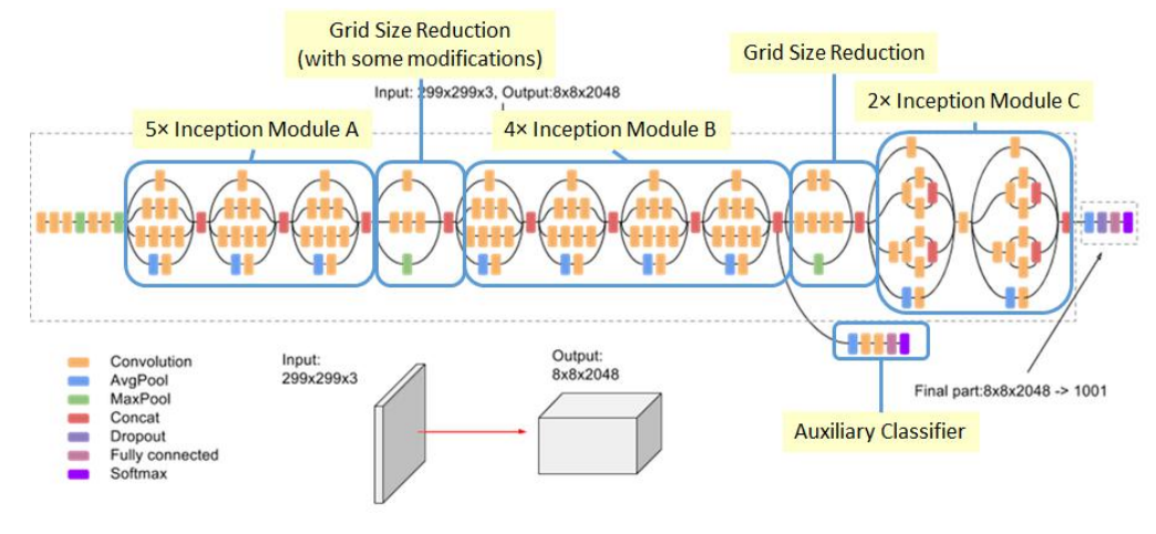
MNIST CNN 示意图

 

• 实战 MNIST CNN 网络

 代码

加载 MNIST 数据集
from keras.datasets import mnist

(x_train, y_train), (x_test, y_test) = mnist.load_data('mnist/mnist.npz')

print(x_train.shape, type(x_train))
print(y_train.shape, type(y_train))
'''
(60000, 28, 28) <class 'numpy.ndarray'>
(60000,) <class 'numpy.ndarray'>
'''

数据处理：规范化

from keras import backend as K

img_rows, img_cols = 28, 28

if K.image_data_format() == 'channels_first':
    x_train = x_train.reshape(x_train.shape[0], 1, img_rows, img_cols)
    x_test = x_test.reshape(x_test.shape[0], 1, img_rows, img_cols)
    input_shape = (1, img_rows, img_cols)
else:
    x_train = x_train.reshape(x_train.shape[0], img_rows, img_cols, 1)
    x_test = x_test.reshape(x_test.shape[0], img_rows, img_cols, 1)
    input_shape = (img_rows, img_cols, 1)


print(x_train.shape, type(x_train))
print(x_test.shape, type(x_test))
'''
(60000, 28, 28, 1) <class 'numpy.ndarray'>
(10000, 28, 28, 1) <class 'numpy.ndarray'>
'''

# 将数据类型转换为float32
X_train = x_train.astype('float32')
X_test = x_test.astype('float32')
# 数据归一化
X_train /= 255
X_test /= 255

print(X_train.shape[0], 'train samples')
print(X_test.shape[0], 'test samples')
'''
60000 train samples
10000 test samples
'''

统计训练数据中各标签数量
import numpy as np
import matplotlib.pyplot as plt

label, count = np.unique(y_train, return_counts=True)
print(label, count)
'''
[0 1 2 3 4 5 6 7 8 9] [5923 6742 5958 6131 5842 5421 5918 6265 5851 5949]
'''

fig = plt.figure()
plt.bar(label, count, width = 0.7, align='center')
plt.title("Label Distribution")
plt.xlabel("Label")
plt.ylabel("Count")
plt.xticks(label)
plt.ylim(0,7500)

for a,b in zip(label, count):
    plt.text(a, b, '%d' % b, ha='center', va='bottom',fontsize=10)

plt.show()

数据处理：one-hot 编码

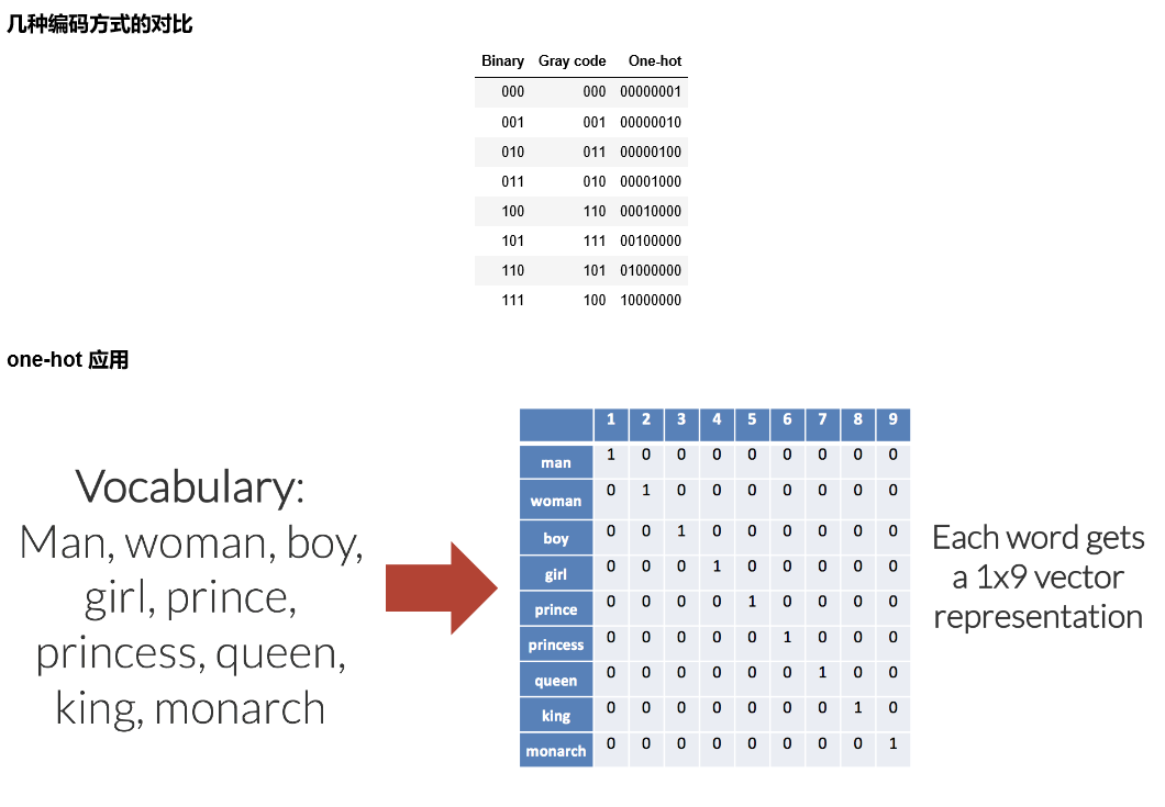
from keras.utils import np_utils

n_classes = 10
print("Shape before one-hot encoding: ", y_train.shape)
Y_train = np_utils.to_categorical(y_train, n_classes)
print("Shape after one-hot encoding: ", Y_train.shape)
Y_test = np_utils.to_categorical(y_test, n_classes)
'''
Shape before one-hot encoding:  (60000,)
Shape after one-hot encoding:  (60000, 10)
'''

print(y_train[0])
print(Y_train[0])
'''
5
[0. 0. 0. 0. 0. 1. 0. 0. 0. 0.]
'''

使用 Keras sequential model 定义 MNIST CNN 网络
from keras.models import Sequential
from keras.layers import Dense, Dropout, Flatten
from keras.layers import Conv2D, MaxPooling2D

model = Sequential()
## Feature Extraction
# 第1层卷积，32个3x3的卷积核 ，激活函数使用 relu
model.add(Conv2D(filters=32, kernel_size=(3, 3), activation='relu',
                 input_shape=input_shape))

# 第2层卷积，64个3x3的卷积核，激活函数使用 relu
model.add(Conv2D(filters=64, kernel_size=(3, 3), activation='relu'))

# 最大池化层，池化窗口 2x2
model.add(MaxPooling2D(pool_size=(2, 2)))

# Dropout 25% 的输入神经元
model.add(Dropout(0.25))

# 将 Pooled feature map 摊平后输入全连接网络
model.add(Flatten())

## Classification
# 全联接层
model.add(Dense(128, activation='relu'))

# Dropout 50% 的输入神经元
model.add(Dropout(0.5))

# 使用 softmax 激活函数做多分类，输出各数字的概率
model.add(Dense(n_classes, activation='softmax'))

查看 MNIST CNN 模型网络结构
model.summary()
'''_________________________________________________________________
Layer (type)                 Output Shape              Param #   
=================================================================
conv2d_1 (Conv2D)            (None, 26, 26, 32)        320       
_________________________________________________________________
conv2d_2 (Conv2D)            (None, 24, 24, 64)        18496     
_________________________________________________________________
max_pooling2d_1 (MaxPooling2 (None, 12, 12, 64)        0         
_________________________________________________________________
dropout_1 (Dropout)          (None, 12, 12, 64)        0         
_________________________________________________________________
flatten_1 (Flatten)          (None, 9216)              0         
_________________________________________________________________
dense_1 (Dense)              (None, 128)               1179776   
_________________________________________________________________
dropout_2 (Dropout)          (None, 128)               0         
_________________________________________________________________
dense_2 (Dense)              (None, 10)                1290      
=================================================================
Total params: 1,199,882
Trainable params: 1,199,882
Non-trainable params: 0
_________________________________________________________________
'''

for layer in model.layers:
    print(layer.get_output_at(0).get_shape().as_list())
'''
[None, 26, 26, 32]
[None, 24, 24, 64]
[None, 12, 12, 64]
[None, 12, 12, 64]
[None, None]
[None, 128]
[None, 128]
[None, 10]
'''

编译模型
model.compile(loss='categorical_crossentropy', metrics=['accuracy'], optimizer='adam')

训练模型，并将指标保存到 history 中

history = model.fit(X_train,
                    Y_train,
                    batch_size=128,
                    epochs=5,
                    verbose=2,
                    validation_data=(X_test, Y_test))
'''
Train on 60000 samples, validate on 10000 samples
Epoch 1/5
 - 64s - loss: 0.2603 - acc: 0.9205 - val_loss: 0.0581 - val_acc: 0.9825
Epoch 2/5
 - 68s - loss: 0.0924 - acc: 0.9729 - val_loss: 0.0420 - val_acc: 0.9855
Epoch 3/5
 - 69s - loss: 0.0714 - acc: 0.9786 - val_loss: 0.0325 - val_acc: 0.9891
Epoch 4/5
 - 68s - loss: 0.0582 - acc: 0.9820 - val_loss: 0.0322 - val_acc: 0.9889
Epoch 5/5
 - 68s - loss: 0.0497 - acc: 0.9849 - val_loss: 0.0310 - val_acc: 0.9900
'''

可视化指标
fig = plt.figure()
plt.subplot(2,1,1)
plt.plot(history.history['acc'])
plt.plot(history.history['val_acc'])
plt.title('Model Accuracy')
plt.ylabel('accuracy')
plt.xlabel('epoch')
plt.legend(['train', 'test'], loc='lower right')

plt.subplot(2,1,2)
plt.plot(history.history['loss'])
plt.plot(history.history['val_loss'])
plt.title('Model Loss')
plt.ylabel('loss')
plt.xlabel('epoch')
plt.legend(['train', 'test'], loc='upper right')
plt.tight_layout()

plt.show()

保存模型

import os
import tensorflow.gfile as gfile

save_dir = "./mnist/model/"

if gfile.Exists(save_dir):
    gfile.DeleteRecursively(save_dir)
gfile.MakeDirs(save_dir)

model_name = 'keras_mnist.h5'
model_path = os.path.join(save_dir, model_name)
model.save(model_path)
print('Saved trained model at %s ' % model_path)
'''
Saved trained model at ./mnist/model/keras_mnist.h5 
'''

加载模型
from keras.models import load_model

mnist_model = load_model(model_path)

统计模型在测试集上的分类结果
loss_and_metrics = mnist_model.evaluate(X_test, Y_test, verbose=2)
    
print("Test Loss: {}".format(loss_and_metrics[0]))
print("Test Accuracy: {}%".format(loss_and_metrics[1]*100))

predicted_classes = mnist_model.predict_classes(X_test)

correct_indices = np.nonzero(predicted_classes == y_test)[0]
# incorrect_indices = np.nonzero(predicted_classes != y_test)[0]
incorrect_indices = np.nonzero(predicted_classes != y_test)
print("Classified correctly count: {}".format(len(correct_indices)))
# print("Classified incorrectly count: {}".format(len(incorrect_indices)))
print("Classified incorrectly count: {}".format(incorrect_indices))
type(incorrect_indices)
'''
Test Loss: 0.03102766538519645
Test Accuracy: 99.0%
Classified correctly count: 9900
Classified incorrectly count: (array([ 321,  582,  659,  674,  717,  740,  947, 1014, 1033, 1039, 1112,
       1182, 1226, 1232, 1242, 1260, 1319, 1326, 1393, 1414, 1527, 1530,
       1549, 1709, 1717, 1737, 1790, 1878, 1901, 2035, 2040, 2043, 2109,
       2118, 2130, 2135, 2293, 2387, 2454, 2462, 2597, 2630, 2654, 2896,
       2921, 2939, 2995, 3005, 3030, 3073, 3422, 3503, 3520, 3558, 3597,
       3727, 3767, 3780, 3808, 3853, 3906, 3941, 3968, 4075, 4176, 4238,
       4248, 4256, 4294, 4497, 4536, 4571, 4639, 4740, 4761, 4807, 4860,
       4956, 5246, 5749, 5937, 5955, 6071, 6091, 6166, 6576, 6597, 6625,
       6651, 6783, 8527, 9009, 9015, 9019, 9024, 9530, 9664, 9729, 9770,
       9982], dtype=int64),)
'''
Out[25]: tuple