

34.62365962451697,78.0246928153624,0
30.28671076822607,43.89499752400101,0
35.84740876993872,72.90219802708364,0
60.18259938620976,86.30855209546826,1
79.0327360507101,75.3443764369103,1
45.08327747668339,56.3163717815305,0
61.10666453684766,96.51142588489624,1
75.02474556738889,46.55401354116538,1
76.09878670226257,87.42056971926803,1
84.43281996120035,43.53339331072109,1
95.86155507093572,38.22527805795094,0
75.01365838958247,30.60326323428011,0
82.30705337399482,76.48196330235604,1
69.36458875970939,97.71869196188608,1
39.53833914367223,76.03681085115882,0
53.9710521485623,89.20735013750205,1
69.07014406283025,52.74046973016765,1
67.94685547711617,46.67857410673128,0
70.66150955499435,92.92713789364831,1
76.97878372747498,47.57596364975532,1
67.37202754570876,42.83843832029179,0
89.67677575072079,65.79936592745237,1
50.534788289883,48.85581152764205,0
34.21206097786789,44.20952859866288,0
77.9240914545704,68.9723599933059,1
62.27101367004632,69.95445795447587,1
80.1901807509566,44.82162893218353,1
93.114388797442,38.80067033713209,0
61.83020602312595,50.25610789244621,0
38.78580379679423,64.99568095539578,0
61.379289447425,72.80788731317097,1
85.40451939411645,57.05198397627122,1
52.10797973193984,63.12762376881715,0
52.04540476831827,69.43286012045222,1
40.23689373545111,71.16774802184875,0
54.63510555424817,52.21388588061123,0
33.91550010906887,98.86943574220611,0
64.17698887494485,80.90806058670817,1
74.78925295941542,41.57341522824434,0
34.1836400264419,75.2377203360134,0
83.90239366249155,56.30804621605327,1
51.54772026906181,46.85629026349976,0
94.44336776917852,65.56892160559052,1
82.36875375713919,40.61825515970618,0
51.04775177128865,45.82270145776001,0
62.22267576120188,52.06099194836679,0
77.19303492601364,70.45820000180959,1
97.77159928000232,86.7278223300282,1
62.07306379667647,96.76882412413983,1
91.56497449807442,88.69629254546599,1
79.94481794066932,74.16311935043758,1
99.2725269292572,60.99903099844988,1
90.54671411399852,43.39060180650027,1
34.52451385320009,60.39634245837173,0
50.2864961189907,49.80453881323059,0
49.58667721632031,59.80895099453265,0
97.64563396007767,68.86157272420604,1
32.57720016809309,95.59854761387875,0
74.24869136721598,69.82457122657193,1
71.79646205863379,78.45356224515052,1
75.3956114656803,85.75993667331619,1
35.28611281526193,47.02051394723416,0
56.25381749711624,39.26147251058019,0
30.05882244669796,49.59297386723685,0
44.66826172480893,66.45008614558913,0
66.56089447242954,41.09209807936973,0
40.45755098375164,97.53518548909936,1
49.07256321908844,51.88321182073966,0
80.27957401466998,92.11606081344084,1
66.74671856944039,60.99139402740988,1
32.72283304060323,43.30717306430063,0
64.0393204150601,78.03168802018232,1
72.34649422579923,96.22759296761404,1
60.45788573918959,73.09499809758037,1
58.84095621726802,75.85844831279042,1
99.82785779692128,72.36925193383885,1
47.26426910848174,88.47586499559782,1
50.45815980285988,75.80985952982456,1
60.45555629271532,42.50840943572217,0
82.22666157785568,42.71987853716458,0
88.9138964166533,69.80378889835472,1
94.83450672430196,45.69430680250754,1
67.31925746917527,66.58935317747915,1
57.23870631569862,59.51428198012956,1
80.36675600171273,90.96014789746954,1
68.46852178591112,85.59430710452014,1
42.0754545384731,78.84478600148043,0
75.47770200533905,90.42453899753964,1
78.63542434898018,96.64742716885644,1
52.34800398794107,60.76950525602592,0
94.09433112516793,77.15910509073893,1
90.44855097096364,87.50879176484702,1
55.48216114069585,35.57070347228866,0
74.49269241843041,84.84513684930135,1
89.84580670720979,45.35828361091658,1
83.48916274498238,48.38028579728175,1
42.2617008099817,87.10385094025457,1
99.31500880510394,68.77540947206617,1
55.34001756003703,64.9319380069486,1
74.77589300092767,89.52981289513276,1
0.051267,0.69956,1
-0.092742,0.68494,1
-0.21371,0.69225,1
-0.375,0.50219,1
-0.51325,0.46564,1
-0.52477,0.2098,1
-0.39804,0.034357,1
-0.30588,-0.19225,1
0.016705,-0.40424,1
0.13191,-0.51389,1
0.38537,-0.56506,1
0.52938,-0.5212,1
0.63882,-0.24342,1
0.73675,-0.18494,1
0.54666,0.48757,1
0.322,0.5826,1
0.16647,0.53874,1
-0.046659,0.81652,1
-0.17339,0.69956,1
-0.47869,0.63377,1
-0.60541,0.59722,1
-0.62846,0.33406,1
-0.59389,0.005117,1
-0.42108,-0.27266,1
-0.11578,-0.39693,1
0.20104,-0.60161,1
0.46601,-0.53582,1
0.67339,-0.53582,1
-0.13882,0.54605,1
-0.29435,0.77997,1
-0.26555,0.96272,1
-0.16187,0.8019,1
-0.17339,0.64839,1
-0.28283,0.47295,1
-0.36348,0.31213,1
-0.30012,0.027047,1
-0.23675,-0.21418,1
-0.06394,-0.18494,1
0.062788,-0.16301,1
0.22984,-0.41155,1
0.2932,-0.2288,1
0.48329,-0.18494,1
0.64459,-0.14108,1
0.46025,0.012427,1
0.6273,0.15863,1
0.57546,0.26827,1
0.72523,0.44371,1
0.22408,0.52412,1
0.44297,0.67032,1
0.322,0.69225,1
0.13767,0.57529,1
-0.0063364,0.39985,1
-0.092742,0.55336,1
-0.20795,0.35599,1
-0.20795,0.17325,1
-0.43836,0.21711,1
-0.21947,-0.016813,1
-0.13882,-0.27266,1
0.18376,0.93348,0
0.22408,0.77997,0
0.29896,0.61915,0
0.50634,0.75804,0
0.61578,0.7288,0
0.60426,0.59722,0
0.76555,0.50219,0
0.92684,0.3633,0
0.82316,0.27558,0
0.96141,0.085526,0
0.93836,0.012427,0
0.86348,-0.082602,0
0.89804,-0.20687,0
0.85196,-0.36769,0
0.82892,-0.5212,0
0.79435,-0.55775,0
0.59274,-0.7405,0
0.51786,-0.5943,0
0.46601,-0.41886,0
0.35081,-0.57968,0
0.28744,-0.76974,0
0.085829,-0.75512,0
0.14919,-0.57968,0
-0.13306,-0.4481,0
-0.40956,-0.41155,0
-0.39228,-0.25804,0
-0.74366,-0.25804,0
-0.69758,0.041667,0
-0.75518,0.2902,0
-0.69758,0.68494,0
-0.4038,0.70687,0
-0.38076,0.91886,0
-0.50749,0.90424,0
-0.54781,0.70687,0
0.10311,0.77997,0
0.057028,0.91886,0
-0.10426,0.99196,0
-0.081221,1.1089,0
0.28744,1.087,0
0.39689,0.82383,0
0.63882,0.88962,0
0.82316,0.66301,0
0.67339,0.64108,0
1.0709,0.10015,0
-0.046659,-0.57968,0
-0.23675,-0.63816,0
-0.15035,-0.36769,0
-0.49021,-0.3019,0
-0.46717,-0.13377,0
-0.28859,-0.060673,0
-0.61118,-0.067982,0
-0.66302,-0.21418,0
-0.59965,-0.41886,0
-0.72638,-0.082602,0
-0.83007,0.31213,0
-0.72062,0.53874,0
-0.59389,0.49488,0
-0.48445,0.99927,0
-0.0063364,0.99927,0
0.63265,-0.030612,0
本次算法的背景是,假如你是一个大学的管理者,你需要根据学生之前的成绩(两门科目)来预测该学生是否能进入该大学。
根据题意,我们不难分辨出这是一种二分类的逻辑回归,输入x有两种(科目1与科目2),输出有两种(能进入本大学与不能进入本大学)。输入测试样例以已经本文最前面贴出分别有两组数据。
我们在进行逻辑回归之前,通常想把数据数据更为直观的显示出来,那么我们根据输入样例绘制图像。
function plotData(X, y)
%PLOTDATA Plots the data points X and y into a new figure
%   PLOTDATA(x,y) plots the data points with + for the positive examples
%   and o for the negative examples. X is assumed to be a Mx2 matrix.

% Create New Figure
figure; hold on;

% ====================== YOUR CODE HERE ======================
% Instructions: Plot the positive and negative examples on a
%               2D plot, using the option 'k+' for the positive
%               examples and 'ko' for the negative examples.


% Find Indices of Positive and Negative Examples
pos = find(y == 1); neg = find(y == 0);
% Plot Examples
plot(X(pos, 1), X(pos, 2), 'k+','LineWidth', 2, 'MarkerSize', 7);
plot(X(neg, 1), X(neg, 2), 'ko', 'MarkerFaceColor', 'y','MarkerSize', 7);


% =========================================================================


hold off;

end
如上代码所展示的是绘图函数,我们可以通过它把数据绘制出来
执行如下代码,绘制图像
clear ; close all; clc

%% Load Data
%  The first two columns contains the exam scores and the third column
%  contains the label.

data = load('ex2data1.txt');
X = data(:, [1, 2]); y = data(:, 3);

%% ==================== Part 1: Plotting ====================
%  We start the exercise by first plotting the data to understand the
%  the problem we are working with.

fprintf(['Plotting data with + indicating (y = 1) examples and o ' ...
         'indicating (y = 0) examples.
']);

plotData(X, y);

% Put some labels
hold on;
% Labels and Legend
xlabel('Exam 1 score')
ylabel('Exam 2 score')

% Specified in plot order
legend('Admitted', 'Not admitted')
hold off;

fprintf('
Program paused. Press enter to continue.
');
pause;
绘制结果入下图所示:
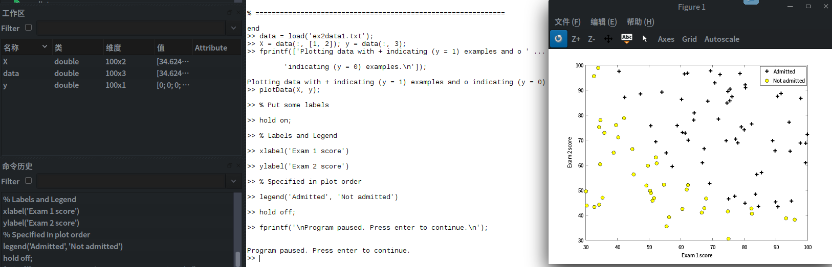
图中用+与O分别表示y = 1 与y = 0的两种结果。
在接触到真正的代价函数之前,我们通常假设函数是hΘ(x)= g(ΘTx)
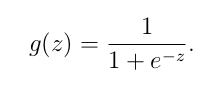
是一S形函数,他可以很好的将0与1区分开。
S形函数的实现:
function g = sigmoid(z)
%SIGMOID Compute sigmoid functoon
%   J = SIGMOID(z) computes the sigmoid of z.

% You need to return the following variables correctly
g = zeros(size(z));

% ====================== YOUR CODE HERE ======================
% Instructions: Compute the sigmoid of each value of z (z can be a matrix,
%               vector or scalar).
g = 1 ./ ( 1 + exp(-z) ) ;
% =============================================================

end
现在我们可以对逻辑函数进行梯度下降,回归函数中的代价函数J(Θ)
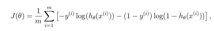
代价函数代码实现为
function [J, grad] = costFunction(theta, X, y)
%COSTFUNCTION Compute cost and gradient for logistic regression
%   J = COSTFUNCTION(theta, X, y) computes the cost of using theta as the
%   parameter for logistic regression and the gradient of the cost
%   w.r.t. to the parameters.

% Initialize some useful values
m = length(y); % number of training examples

% You need to return the following variables correctly
J = 0;
grad = zeros(size(theta));

% ====================== YOUR CODE HERE ======================
% Instructions: Compute the cost of a particular choice of theta.
%               You should set J to the cost.
%               Compute the partial derivatives and set grad to the partial
%               derivatives of the cost w.r.t. each parameter in theta
%
% Note: grad should have the same dimensions as theta
%

J= -1 * sum( y .* log( sigmoid(X*theta) ) + (1 - y ) .* log( (1 - sigmoid(X*theta)) ) ) / m ;

grad = ( X' * (sigmoid(X*theta) - y ) )/ m ;


% =============================================================

end
function [J, grad] = costFunctionReg(theta, X, y, lambda)
%COSTFUNCTIONREG Compute cost and gradient for logistic regression with regularization
%   J = COSTFUNCTIONREG(theta, X, y, lambda) computes the cost of using
%   theta as the parameter for regularized logistic regression and the
%   gradient of the cost w.r.t. to the parameters.

% Initialize some useful values
m = length(y); % number of training examples

% You need to return the following variables correctly
J = 0;
grad = zeros(size(theta));

% ====================== YOUR CODE HERE ======================
% Instructions: Compute the cost of a particular choice of theta.
%               You should set J to the cost.
%               Compute the partial derivatives and set grad to the partial
%               derivatives of the cost w.r.t. each parameter in theta

theta_1=[0;theta(2:end)];
J= -1 * sum( y .* log( sigmoid(X*theta) ) + (1 - y ) .* log( (1 - sigmoid(X*theta)) ) ) / m  + lambda/(2*m) * theta_1' * theta_1 ;
grad = ( X' * (sigmoid(X*theta) - y ) )/ m + lambda/m * theta_1 ;


% =============================================================

end
预测函数:
function p = predict(theta, X)
%PREDICT Predict whether the label is 0 or 1 using learned logistic
%regression parameters theta
%   p = PREDICT(theta, X) computes the predictions for X using a
%   threshold at 0.5 (i.e., if sigmoid(theta'*x) >= 0.5, predict 1)

m = size(X, 1); % Number of training examples

% You need to return the following variables correctly
p = zeros(m, 1);

% ====================== YOUR CODE HERE ======================
% Instructions: Complete the following code to make predictions using
%               your learned logistic regression parameters.
%               You should set p to a vector of 0's and 1's
%

k = find(sigmoid( X * theta) >= 0.5 );
p(k)= 1;

% p(sigmoid( X * theta) >= 0.5) = 1;   % it's a more compat way.


% =========================================================================


end
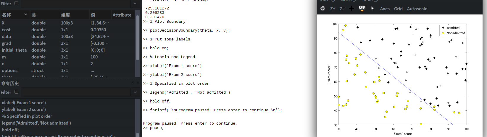
现在我们实现代价函数和他的梯度下降,并拟合出直线
%% ============ Part 2: Compute Cost and Gradient ============
%  In this part of the exercise, you will implement the cost and gradient
%  for logistic regression. You neeed to complete the code in
%  costFunction.m

%  Setup the data matrix appropriately, and add ones for the intercept term
[m, n] = size(X);

% Add intercept term to x and X_test
X = [ones(m, 1) X];

% Initialize fitting parameters
initial_theta = zeros(n + 1, 1);

% Compute and display initial cost and gradient
[cost, grad] = costFunction(initial_theta, X, y);

fprintf('Cost at initial theta (zeros): %f
', cost);
fprintf('Gradient at initial theta (zeros):
');
fprintf(' %f
', grad);

fprintf('
Program paused. Press enter to continue.
');
pause;
%% ============= Part 3: Optimizing using fminunc  =============
%  In this exercise, you will use a built-in function (fminunc) to find the
%  optimal parameters theta.

%  Set options for fminunc
options = optimset('GradObj', 'on', 'MaxIter', 400);

%  Run fminunc to obtain the optimal theta
%  This function will return theta and the cost
[theta, cost] = ...
	fminunc(@(t)(costFunction(t, X, y)), initial_theta, options);

% Print theta to screen
fprintf('Cost at theta found by fminunc: %f
', cost);
fprintf('theta:
');
fprintf(' %f
', theta);

% Plot Boundary
plotDecisionBoundary(theta, X, y);

% Put some labels
hold on;
% Labels and Legend
xlabel('Exam 1 score')
ylabel('Exam 2 score')

% Specified in plot order
legend('Admitted', 'Not admitted')
hold off;

fprintf('
Program paused. Press enter to continue.
');
pause;

%% ============== Part 4: Predict and Accuracies ==============
%  After learning the parameters, you'll like to use it to predict the outcomes
%  on unseen data. In this part, you will use the logistic regression model
%  to predict the probability that a student with score 45 on exam 1 and
%  score 85 on exam 2 will be admitted.
%
%  Furthermore, you will compute the training and test set accuracies of
%  our model.
%
%  Your task is to complete the code in predict.m

%  Predict probability for a student with score 45 on exam 1
%  and score 85 on exam 2

prob = sigmoid([1 45 85] * theta);
fprintf(['For a student with scores 45 and 85, we predict an admission ' ...
         'probability of %f

'], prob);

% Compute accuracy on our training set
p = predict(theta, X);

fprintf('Train Accuracy: %f
', mean(double(p == y)) * 100);

fprintf('
Program paused. Press enter to continue.
');
pause;
实例2,对非线性函数进行逻辑回归,
实现步骤如下:
%% Machine Learning Online Class - Exercise 2: Logistic Regression
%
%  Instructions
%  ------------
%
%  This file contains code that helps you get started on the second part
%  of the exercise which covers regularization with logistic regression.
%
%  You will need to complete the following functions in this exericse:
%
%     sigmoid.m
%     costFunction.m
%     predict.m
%     costFunctionReg.m
%
%  For this exercise, you will not need to change any code in this file,
%  or any other files other than those mentioned above.
%

%% Initialization
clear ; close all; clc

%% Load Data
%  The first two columns contains the X values and the third column
%  contains the label (y).

data = load('ex2data2.txt');
X = data(:, [1, 2]); y = data(:, 3);

plotData(X, y);

% Put some labels
hold on;

% Labels and Legend
xlabel('Microchip Test 1')
ylabel('Microchip Test 2')

% Specified in plot order
legend('y = 1', 'y = 0')
hold off;


%% =========== Part 1: Regularized Logistic Regression ============
%  In this part, you are given a dataset with data points that are not
%  linearly separable. However, you would still like to use logistic
%  regression to classify the data points.
%
%  To do so, you introduce more features to use -- in particular, you add
%  polynomial features to our data matrix (similar to polynomial
%  regression).
%

% Add Polynomial Features

% Note that mapFeature also adds a column of ones for us, so the intercept
% term is handled
X = mapFeature(X(:,1), X(:,2));

% Initialize fitting parameters
initial_theta = zeros(size(X, 2), 1);

% Set regularization parameter lambda to 1
lambda = 1;

% Compute and display initial cost and gradient for regularized logistic
% regression
[cost, grad] = costFunctionReg(initial_theta, X, y, lambda);

fprintf('Cost at initial theta (zeros): %f
', cost);

fprintf('
Program paused. Press enter to continue.
');
pause;

%% ============= Part 2: Regularization and Accuracies =============
%  Optional Exercise:
%  In this part, you will get to try different values of lambda and
%  see how regularization affects the decision coundart
%
%  Try the following values of lambda (0, 1, 10, 100).
%
%  How does the decision boundary change when you vary lambda? How does
%  the training set accuracy vary?
%

% Initialize fitting parameters
initial_theta = zeros(size(X, 2), 1);

% Set regularization parameter lambda to 1 (you should vary this)
lambda = 1;

% Set Options
options = optimset('GradObj', 'on', 'MaxIter', 400);

% Optimize
[theta, J, exit_flag] = ...
	fminunc(@(t)(costFunctionReg(t, X, y, lambda)), initial_theta, options);

% Plot Boundary
plotDecisionBoundary(theta, X, y);
hold on;
title(sprintf('lambda = %g', lambda))

% Labels and Legend
xlabel('Microchip Test 1')
ylabel('Microchip Test 2')

legend('y = 1', 'y = 0', 'Decision boundary')
hold off;

% Compute accuracy on our training set
p = predict(theta, X);

fprintf('Train Accuracy: %f
', mean(double(p == y)) * 100);
样本:

逻辑回归:
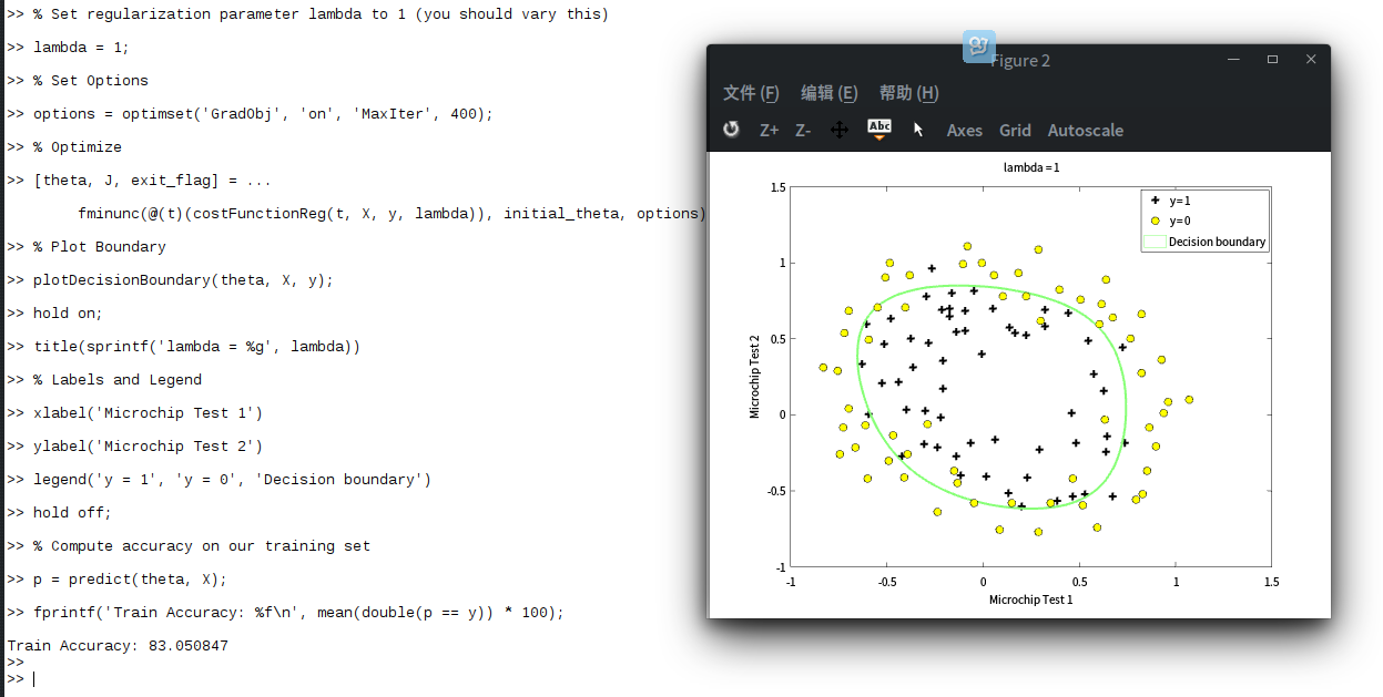
预测结果:为83.050847