Pytorch04_RNN结构

RNN结构

本文中的RNN泛指LSTM，GRU等等
CNN中和RNN中batchSize的默认位置是不同的。

CNN中：batchsize 的位置是 position 0.

RNN中：batchsize 的位置是 position 1.

一、pytorch中两种调取方式

对于最简单的RNN，我们可以使用两种方式来调用.

torch.nn.RNNCell()    它只接受序列中的单步输入，必须显式的传入隐藏状态。

torch.nn.RNN()    可以接受一个序列的输入，默认会传入一个全0的隐藏状态，也可以自己申明隐藏状态传入。

RNN结构及隐藏状态是什么参考下文 https://www.cnblogs.com/Haozi-D17/p/13264745.html

二、参数及输入输出结构

输入大小

输入大小是三维tensor[seq_len,batch_size,input_dim]

input_dim 是输入的维度 或者说是 数据的特征数，比如是128
batch_size 是一次往RNN输入句子的数目 或者说是 有几组独立的输入数据，比如是5。
seq_len 是一个句子的最大长度 或者说是 每组训练数据的时间长度，比如15

输入顺序

注意，RNN输入的是序列，一次把批次的所有句子都输入了，得到的 ouptut 和 hidden 都是这个批次的所有的输出和隐藏状态，维度也是三维。
可以理解为现在一共有 batch_size 个独立的 RNN 组件，RNN的输入维度是 input_dim，总共输入 seq_len 个时间步，则每个时间步输入到这个整个RNN模块的维度是 [batch_size,input_dim]

将 seq_len 放在第一位的好处是，可以同时处理每个句子

1. 第一个时间步，输入所有句子的第一个单词 或者 第一个时间上的所有特征；

2. 第二个时间步，输入所有句子的第二个单词 或者 第二个时间上的所有特征；

...

3. 以此类推，直到 seq_len 个时间步全部输入完成。

举例

# 构造RNN网络，x的维度5，隐层的维度10,网络的层数2
rnn_seq = nn.RNN(5, 10,2)  
# 构造一个输入序列，句长为 6，batch 是 3， 每个单词使用长度是 5的向量表示
x = torch.randn(6, 3, 5)
#out,ht = rnn_seq(x,h0) 
out,ht = rnn_seq(x) #h0可以指定或者不指定

问题1：这里 out、ht 的 size 是多少呢？
回答：out: 6 * 3 * 10, ht: 2 * 3 * 10，out 的输出维度 [seq_len,batch_size,output_dim]，ht 的维度 [num_layers * num_directions, batch_size, hidden_size], 如果是单向单层的 RNN 那么一个句子只有一个 hidden。
问题2：out[-1] 和 ht[-1] 是否相等？
回答：相等，隐藏单元就是输出的最后一个单元，可以想象，每个的输出其实就是那个时间步的隐藏单元

 可以想象 当 input 为 [seq_len,batch_size,input_dim] 时：

out 的 维度 即为 将输入每个时间步上的 特征做了映射，因此只改变最后一个维度，得到的结果即为 [seq_len, batch_size, output_dim]

ht 的 第一个维度 与句子长度无关，因为只是在不断改变和更新的过程，但方向和层数 会影响，为num_layers * num_directions。

　　第二个维度为batch_size，有几个句子就得到几个维度。

　　最后一个维度同 out 的维度变换，为 hidden_size 

　　ht 的维度 [num_layers * num_directions, batch_size, hidden_size]

但 out[-1] = ht[-1]（上述代码中），是因为 ht 最终 只保存最后一个时刻的值

RNN的其他参数

nn.RNN(input_dim ,hidden_dim ,num_layers ，…)
– input_dim 表示输入的特征维度
– hidden_dim 表示输出的特征维度，如果没有特殊变化，相当于out
– num_layers 表示网络的层数
– nonlinearity 表示选用的非线性**函数，默认是 ‘tanh’
– bias 表示是否使用偏置，默认使用
– batch_first 表示输入数据的形式，默认是 False，就是这样形式，(seq, batch, feature)，也就是将序列长度放在第一位，batch 放在第二位
– dropout 表示是否在输出层应用 dropout
– bidirectional 表示是否使用双向的 rnn，默认是 False

LSTM

LSTM的输出相比于GRU多了一个memory单元

# 输入维度 50，隐层100维，两层
lstm_seq = nn.LSTM(50, 100, num_layers=2)
# 输入序列seq= 10，batch =3，输入维度=50
lstm_input = torch.randn(10, 3, 50)
out, (h, c) = lstm_seq(lstm_input) # 使用默认的全 0 隐藏状态

问题1：out和(h,c)的size各是多少？
回答：out：(10 * 3 * 100)，(h,c)：都是(2 * 3 * 100)
问题2：out[-1,:,:]和h[-1,:,:]相等吗？
回答： 相等
GRU比较像传统的RNN

gru_seq = nn.GRU(10, 20,2) # x_dim,h_dim,layer_num
gru_input = torch.randn(3, 32, 10) # seq，batch，x_dim
out, h = gru_seq(gru_input)

三、代码案例

以一个时间序列预测为例。代码以先后顺序写，直接按顺序复制即可运行。

首先，导入库

import numpy as np
import pandas as pd
import matplotlib.pyplot as plt
import torch

演示一下我们需要做的事，这部分不用再自己的代码中跑，单纯演示

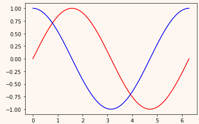
steps = np.linspace(0, np.pi*2, 100, dtype=np.float32)
x = np.sin(steps)
y = np.cos(steps)
plt.plot(steps, x, "r-")
plt.plot(steps, y, "b-")
plt.show()

如下图，输入为红色的线上的点，想要输出为对应的蓝色的点，即用 sin上的点 预测 同样位置的 cos 上的点

生成所用数据 x 和 y 

train_x = np.zeros(shape=(100, 10, 1))
train_y = np.zeros(shape=(100, 10))         
for step in range(100):
    start, end = step * np.pi, (step+1)*np.pi
    steps = np.linspace(start, end, 10, dtype=np.float32)
    train_x[step,:,0] = np.sin(steps)    # float32 for converting torch FloatTensor
    train_y[step,:] = np.cos(steps)

# 转换为张量
train_x = torch.from_numpy(train_x)
train_y = torch.from_numpy(train_y)

train_x 为 一条 sin 曲线，shape 为 (100, 10, 1)

train_y 为 一条 cos 曲线，shape 为 (100, 10)

将 x 和 y 打包为数据集

其中：

　　32 表示从中取数据的时候每次取出32组（一共有100组）

　　shuffle=True 表示取数据的时候 将100组数据打乱，随机取

　　num_workers = 2 表示使用多线程

import torch.utils.data as Data
torch_dataset = Data.TensorDataset(train_x, train_y)

loader = Data.DataLoader(
    dataset=torch_dataset,
    batch_size=32,
    shuffle=True,  # 每次训练打乱数据， 默认为False
    num_workers=2,  # 使用多进行程读取数据， 默认0，为不使用多进程
    )

构建 GRU 模型

import  torch.nn as nn
import  torch.optim as optim

# 搭建模型
input_size = 1
hidden_size = 16
output_size = 10
num_layers = 1

class GRU(nn.Module):
    def __init__(self, ):
        super(GRU, self).__init__()
        self.gru = nn.GRU(input_size=input_size, # feature_len=1
                          hidden_size=hidden_size, # 隐藏记忆单元尺寸hidden_len
                          num_layers=num_layers,      #层数
                          batch_first=True,      # 在传入数据时,按照[batch,seq_len,feature_len]的格式
                         )
        self.linear = nn.Linear(hidden_size, output_size)  #输出层

    def forward(self, x):
        out, h_t = self.gru(x)  # out(batch, seq_len, feature_len)
        # 思路一：将out的所有结果 都输到 linear，再取最后一个
        # 因为要将out输入linear，因此先将batch和time_step打平
#         out = out.reshape(-1, hidden_size) # [batch,seq_len,hidden_len]->[batch*seq_len,hidden_len]
#         out = self.linear(out)  # [batch*seq_len,hidden_len]
#         out = out.unsqueeze(dim=0) # 增加一个维度batch [seq_len,feature_len]->[batch=1,seq_len,feature_len]
#         out = out.reshape(-1, 10, output_size) # 重新恢复为原来的维度（最后一个维度变了）
#         out = out[:, -1, :]  # 只取最后一个  取出的out.shape为 torch.Size([batch, output_size])
        # 思路二：直接取out的最后一个时间维度的结果输入到 linear
        out = out[:, -1, :]
        out = self.linear(out)
        
        return out

batch_first=True，如开头所说，默认的输入应该为 [seq_len, batch, feature_len], 此参数设为True，表示输入为[batch，seq_len, feature_len]

设置优化器和损失计算函数

model = GRU().cuda()  # 若不用GPU 删掉.cuda()即可
criterion = nn.MSELoss()
optimizer = optim.Adam(model.parameters(), lr=1e-2)

训练

for epoch in range(100):
    for step, (batch_x, batch_y) in enumerate(loader):
        x = batch_x.float().cuda()
        y = batch_y.float().cuda() # .reshape(-1, 1, Out).cuda()
        output = model(x)
        loss = criterion(output, y).cuda()
        model.zero_grad()
        loss.backward(retain_graph=True) # 
        optimizer.step()

    if epoch: #  % 100 == 0:
        print("Epoch: ", epoch, "| Loss: ", loss.item())
    
    # 展示结果的地方解释这段
    # pre = model(train_x.float().cuda())
    # plt.plot(pre[0,:].cpu().detach().numpy(), c="r")
    # plt.plot(train_y[0,:], c="b")
    # plt.show()

将训练用的 x 重新输入得到预测结果

pre = model(train_x.float().cuda())
print(pre)

效果展示

　　任意比较一组预测值与实际值，若想比较所有的值，将预测的100组连起来就好了。

　　上面预测的数据在GPU上存着，画图需要在cpu上复制一份数据，并转换为numpy 才能在cpu上画图

plt.plot(pre[0,:].cpu().detach().numpy(), c="r")
plt.plot(train_y[0,:], c="b")

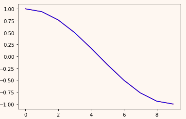
可以看出，基本重合

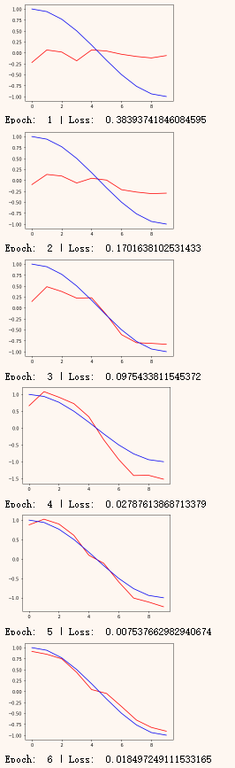
下图表示动态变化，可以看出没用几次就可以训练的很好了。

　　就是训练的代码框里最后注释掉的一段，如果不注释就会看到训练的效果（方法比较简单，有更好的方法，可以自己搜一下）