python一对一教程：Computational Problems for Physics chapter 1-B Code Listings 1.7

作者自我介绍：大爽歌, b站小UP主，直播编程+红警三，python1对1辅导老师。
本博客为一对一辅导学生python代码的教案, 获得学生允许公开。
具体辅导内容为《Computational Problems for Physics With Guided Solutions Using Python》，第一章（Chapter 1 Computational Basics for Physics）的 Code Listings
由于代码较多，第一章内容分为三部分
A(1.1 - 1.6)
B(1.7 - 1.12)
C(1.12 - 1.17)

1 - 1.7 PondMatPlot.py

1 subplots

Create a figure and a set of subplots.
subplots() without arguments returns a Figure and a single Axes.

创建一个图形(figure)和一组子图(ax)。
如果没有参数，返回单个图形和单个轴。

ax: an .axes.Axes or array of Axes

2 `.axes.Axes` 的方法

官方文档： axes_api

set_xlabel
set_ylabel

这两个方法很简单，就是设置标签，只不过这里用到了一个参数fontsize，代表标签字体大小。
详细参数列表见Text的 Valid keyword arguments

set_xlim
set_ylim

设置x轴，y轴视图限制。即设置轴的范围（两个端点大小）

支持以下写法（set_ylim同理）,以下两种写法一个意思。

set_xlim(left, right)
set_xlim((left, right))

set_xticks(ticks) 设置xaxis的刻度位置。

ticks: List of tick locations(floats).

set_xticklabels(labels) 用字符串标签列表设置xaxis的标签。

labels: list of label texts(str).

补充说明：set_xticklabels使用前，必须先调用set_xticks，且ticks和labels元素个数要一致。

3 PondMatPlot 绘制效果

import numpy as np, matplotlib.pyplot as plt

N = 100;   Npts = 3000;  analyt = np.pi**2                                      
x1 = np.arange(0, 2*np.pi+2*np.pi/N,2*np.pi/N)   
xi = [];  yi = [];  xo = [];  yo = []   
fig,ax = plt.subplots()
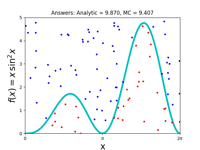
y1 = x1 * np.sin(x1)**2                           # Integrand
ax.plot(x1, y1, 'c', linewidth=4)      
ax.set_xlim ((0, 2*np.pi))
ax.set_ylim((0, 5))
ax.set_xticks([0, np.pi, 2*np.pi])     
ax.set_xticklabels(['0', '$pi$','2$pi$'])
ax.set_ylabel('$f(x) = x\,sin^2 x$', fontsize=20) 
ax.set_xlabel('x',fontsize=20)
fig.patch.set_visible(False)
   
def fx(x):   return x*np.sin(x)**2                  # Integrand
            
j = 0                                    # Inside curve counter
xx = 2.* np.pi * np.random.rand(Npts)          # 0 =< x <= 2pi
yy = 5*np.random.rand(Npts)                      # 0 =< y <= 5
for i in range(1,Npts):            
    if (yy[i] <= fx(xx[i])):                     # Below curve
        if (i <=100): xi.append(xx[i])               
        if (i <=100): yi.append(yy[i])
        j +=1                            
    else:                           
        if (i <=100): yo.append(yy[i])               
        if (i <=100): xo.append(xx[i])
    boxarea = 2. * np.pi *5.                         # Box area 
    area = boxarea*j/(Npts-1)                # Area under curve

ax.plot(xo,yo,'bo',markersize=3)
ax.plot(xi,yi,'ro',markersize=3)
ax.set_title('Answers: Analytic = %5.3f, MC = %5.3f'%(analyt,area))
plt.show()

效果如图

4 PondMatPlot 逐行解析

N = 100;   Npts = 3000;  analyt = np.pi**2                                      
x1 = np.arange(0, 2*np.pi+2*np.pi/N,2*np.pi/N)

x1 是从0到(2+2/N)pi，等分取的N+1个值组成的数组

ax.plot(x1, y1, 'c', linewidth=4)

绘制颜色为cyan(青色)，线宽为4的曲线

fig.patch.set_visible(False)

将fig背景设为透明，在窗口上看起来和白色没区别，保存成png能看到效果。

def fx(x):   return x*np.sin(x)**2

定义一个函数，对应上面绘制的曲线，方便计算对应的值。

xx = 2.* np.pi * np.random.rand(Npts)  # 0 =< x <= 2pi
yy = 5*np.random.rand(Npts)

np.random.rand(d0, d1, ..., dn)
创建给定形状的数组，并用[0,1)中均匀分布的随机样本填充它。

d0, d1, ..., dn，有几个，数组就是几维。
每个维度的长度由对应的di决定。

所以上面两行代码是在对应的区间内，Npts个[0,1)之中的随机值组成的一维数组。

for i in range(1,Npts):            
    if (yy[i] <= fx(xx[i])):                     # Below curve
        if (i <=100): xi.append(xx[i])               
        if (i <=100): yi.append(yy[i])
        j +=1                            
    else:                           
        if (i <=100): yo.append(yy[i])               
        if (i <=100): xo.append(xx[i])

遍历刚才生成的随机数，如果一组x，y在曲线下面（包括曲线），就放到xi, yi 中。

同时计数器j加1。（j用于统计有多个在曲线下的点）

如果一组x，y在曲线上面，就放到xo, yo中。

boxarea = 2. * np.pi *5.                         # Box area 
area = boxarea*j/(Npts-1)                # Area under curve

根据随机生成的点中，在曲线下的点的数量占比，因为数量足够多，可近似认为其为面积占比。

去计算曲线下的区域面积。

ax.plot(xo,yo,'bo',markersize=3)
ax.plot(xi,yi,'ro',markersize=3)

曲线上的点用蓝色圆点进行绘制，曲线下面的点用红色圆点进行绘制。
圆点的尺寸设置为3。

2 - 1.8 PondMatPlot.py

1 PondMatPlot绘制效果

代码如下

import numpy as np
# from mpl_toolkits.mplot3d import Axes3D
import matplotlib.pyplot as plt

def randrange(n, vmin, vmax):
    return (vmax-vmin)*np.random.rand(n) + vmin

fig = plt.figure()
ax = fig.add_subplot(111, projection='3d')
n = 100
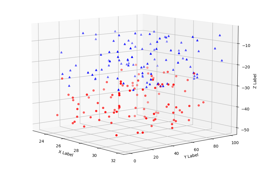
for c, m, zl, zh in [('r', 'o', -50, -25), ('b', '^', -30, -5)]:
    xs = randrange(n, 23, 32)
    ys = randrange(n, 0, 100)
    zs = randrange(n, zl, zh)
    ax.scatter(xs, ys, zs, c=c, marker=m)
ax.set_xlabel('X Label')
ax.set_ylabel('Y Label')
ax.set_zlabel('Z Label')
plt.show()

绘制效果如图

2 fig.add_subplot

fig = plt.figure()
ax = fig.add_subplot(111, projection='3d')

fig.add_subplot
常见参数写法为

(nrows, ncols, index, **kwargs)
(add_subplot(pos, **kwargs)

这里遇到的就是第二种，pos是111，等价于第一种的
nrows=1, ncols=1, index=1。

projection设置子图轴(subplot Axes)的投影类型(projection type)。
这里值为3d代表轴的类型为Axes3D

补充，轴的投影类型，可取值和对应的类型如下

{
    None: "use default",  # The default None results in a 'rectilinear' projection.
    'rectilinear': axes.Axes, 
    'aitoff': AitoffAxes,
    'hammer': HammerAxes, 
    'lambert': LambertAxes, 
    'mollweide': MollweideAxes, 
    'polar': PolarAxes, 
    '3d': Axes3D, 
    str:  "a custom projection",  # see projections. 
}

3 代码逐行解析

def randrange(n, vmin, vmax):
    return (vmax-vmin)*np.random.rand(n) + vmin

定义一个函数，返回一个一维n元，在[vmin, vmax)区间随机分布的数组

n = 100
for c, m, zl, zh in [('r', 'o', -50, -25), ('b', '^', -30, -5)]:
    xs = randrange(n, 23, 32)
    ys = randrange(n, 0, 100)
    zs = randrange(n, zl, zh)
    ax.scatter(xs, ys, zs, c=c, marker=m)

遇到这种循环不好看明白的话，就把这拆开看

n = 100

c, m, zl, zh = ('r', 'o', -50, -25)
xs = randrange(n, 23, 32)
ys = randrange(n, 0, 100)
zs = randrange(n, zl, zh)
ax.scatter(xs, ys, zs, c=c, marker=m)


c, m, zl, zh = ('b', '^', -30, -5)
xs = randrange(n, 23, 32)
ys = randrange(n, 0, 100)
zs = randrange(n, zl, zh)
ax.scatter(xs, ys, zs, c=c, marker=m)

可以看到，就是绘制了两次散点图，

相同点

xs范围相同，23 - 32 之间随机取出n个
ys范围相同，0 - 100 之间随机取出n个

不同点

zs范围不同，
第一次在-50, -25之间随机取出n个；
第二次是在-30, -5之间随机取出n个。
c不同（color不同）
第一次是r红色；
第二次是b蓝色。
marker不同
第一次是o小圆点
第二次是^小三角。

3 - Vpython 再解读

1 `canvas`

对应Vpython6中的display

scene=canvas(heigth=600,width=600,range=380)

doc: https://www.glowscript.org/docs/VPythonDocs/canvas.html
Creates a canvas with the specified attributes, makes it the selected canvas, and returns it.

创建具有指定属性的画布，使其成为选中的画布，并返回它。

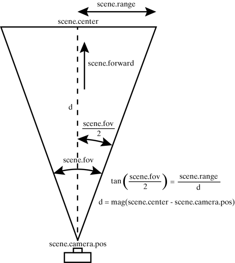
range: The extent of the region of interest to the left or right of center.
受关注区域到中心左右侧的距离

官方文档示意图如下

2 `curve`

doc: https://www.glowscript.org/docs/VPythonDocs/curve.html
The curve object displays straight lines between points, and if the points are sufficiently close together you get the appearance of a smooth curve.
curve展示点组成的直线。

以下写法效果相同，都会绘制v1到v2的曲线(v1, v2为三维坐标向量)

# 1)
c = curve(v1,v2)

# 2)
c = curve([v1,v2])

# 3)
c = curve(pos=[v1,v2])

# 4)
c = curve(v1)
c.append(v2)

# 5)
c = curve()
c.append(v1,v2)

curve还支持设置一些属性，比如

color
radius

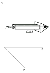
3 `cylinder`

doc: https://www.glowscript.org/docs/VPythonDocs/cylinder.html
cylinder展示一个圆柱体（杆）。

示例

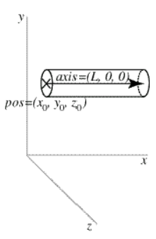
rod = cylinder(pos=vector(0,2,1), axis=vector(5,0,0), radius=1)

pos: the center of one end of the cylinder; default = vector(0,0,0)
圆柱体底端的中心
axis: The axis points from pos to the other end of the cylinder, default = vector(1,0,0). Setting the axis makes length and size.x equal to the magnitude of the axis.
轴从pos点指向圆柱的另一端，设置轴的大小可以决定length和size.x。

官方文档示例图如下

用cylinder创建实例后，可以通过修改实例的属性值，修改其状态，
比如修改其pos和axis。

其他属性(代码中用到的)

color
radius

4 `arrow`

doc: https://www.glowscript.org/docs/VPythonDocs/arrow.html

创建一端带有箭头的盒形直轴的箭头对象。
示例

pointer = arrow(pos=vector(0,2,1), axis=vector(5,0,0))

pos
axis

两参数效果见下官方示意图

5 `label`

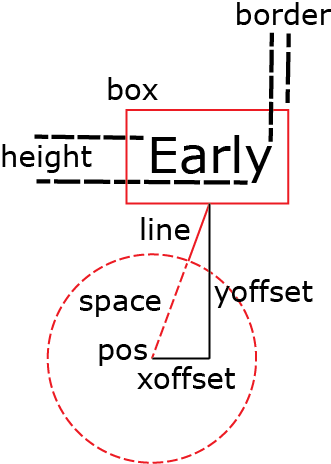
doc: https://www.glowscript.org/docs/VPythonDocs/label.html

使用label对象，可以在一个框中显示文本，
示例

label(pos=vec(0,0.25,0), text='Hello!', box=0)

text: 标签框中的文本，字符串，支持html语法。
pos: 用于标签框底部中间位置(xoffset, yoffset为0时)
box: 默认为True，代表方框应该被绘制。False则不会绘制，（0等价于False,1为True）

参数详细官方示意图如下

生成label实例后，可修改实例的属性，调整对应标签的展示效果。

6 `local_light`

doc: https://www.glowscript.org/docs/VPythonDocs/lights.html
You can light a scene with distant lights (which act like point-like lamps far from the scene) and/or local lights (point-like lamps near the scene).

可以使用远光源（其作用类似于远离场景的点光源）和/或局部光源（靠近场景的点光源）照亮场景。

scene的默认灯光设置scene.lights如下

[distant_light(direction=vector( 0.22,  0.44,  0.88),       color=color.gray(0.8)),
 distant_light(direction=vector(-0.88, -0.22, -0.44),       color=color.gray(0.3))]

创建局部光源代码示例

lamp = local_light(pos=vector(x,y,z), color=color.yellow)

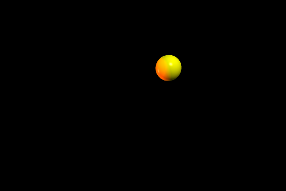
这里举一个展示光源移动的效果代码

from vpython import *

scene=canvas(heigth=600,width=600,range=380)
sball = sphere(pos=vector(100, 100, 0), radius=50, color=color.yellow)

X = -300
lamp = local_light(pos=vector(X, 0, 0), color=color.red)   # light

for t in arange(0.,100.0,0.2):
    rate(50)
    MX = X + t * 6
    lamp.pos = vector(MX, 0, 20)

其效果如下图

7 `rate`

设置动画一秒刷新的次数，动画的帧数，放在循环里就会调整循环一秒执行的次数。

Halts computations until 1.0/frequency seconds after the previous call to rate().
具体效果为，调用rate(frequency)将会停止运算 1.0/frequency 秒
doc: https://www.glowscript.org/docs/VPythonDocs/rate.html

4 - 1.9 TwoForces.py

1 为Vpython7更新代码语法

首先说明，1.9 TwoForces.py 是用Classic VPython (VPython 6)。
部分语法Vpython7中已经不支持。
其语法改换成Vpython7后代码如下

from vpython import *  # TwoForces.py

posy=100;  Lcord=250  # basic height, cord length
Hweight=50;  W = 10   # cylinder height, weight 

scene=canvas(heigth=600,width=600,range=380)
alt=curve(pos=[(-300,posy,0),(300,posy,0)])
divi=curve(pos=[(0,-150,0),(0,posy,0)])
kilogr=cylinder(pos=vector(0,posy-Lcord,0),radius=20,axis=vector(0,-Hweight,0),
                color=color.red) # kg as a cylinder
cord1=cylinder(pos=vector(0,posy,0),axis=vector(0,-Lcord,0),color=color.yellow,
               radius=2)
cord2=cylinder(pos=vector(0,posy,0),axis=vector(0,-Lcord,0),color=color.yellow,
               radius=2)

arrow1=arrow(pos=vector(0,posy,0), color=color.orange) # Tension cord 1
arrow2=arrow(pos=vector(0,posy,0), color=color.orange) # Tension cord 2

magF=W/2.0          # initial force of each student
v=2.0               # (m/s) velocity of each student
x1=0.0              # initial position student 1
anglabel=label(pos=vector(0,240,0), text='angle (deg)',box=0)
angultext=label(pos=vector(20,210,0),box=0)
Flabel1=label(pos=vector(200,240,0), text='Force',box=0)
Ftext1=label(pos=vector(200,210,0),box=0)
Flabel2=label(pos=vector(-200,240,0), text='Force',box=0)
Ftext2=label(pos=vector(-200,210,0),box=0)
local_light(pos=vector(-10,0,20), color=color.yellow)   # light

for t in arange(0.,100.0,0.2):  
    rate(50)                  # slow motion
    x1=v*t                    # 1 to right, 2 to left
    theta=asin(x1/Lcord)      # angle cord
    poscil=posy-Lcord*cos(theta)  # cylinder height
    kilogr.pos=vector(0,poscil,0)     # y-position kilogram
    magF=W/(2.*cos(theta))      # Cord tension
    angle=180.*theta/pi     
    cord1.pos=vector(x1,posy,0)       # position cord end
    cord1.axis=vector(-Lcord*sin(theta),-Lcord*cos(theta),0)
    cord2.pos=vector(-x1,posy,0)            # position end cord
    cord2.axis=vector(Lcord*sin(theta),-Lcord*cos(theta),0)
    arrow1.pos=cord1.pos            # axis arrow 
    arrow1.axis=vector(8*magF*sin(theta),8*magF*cos(theta),0)
    arrow2.pos=cord2.pos
    arrow2.axis=vector(-8*magF*sin(theta),8*magF*cos(theta),0)
    angultext.text='%4.2f'%angle
    force=magF
    Ftext1.text='%8.2f'%force     # Tension
    Ftext2.text='%8.2f'%force

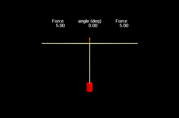
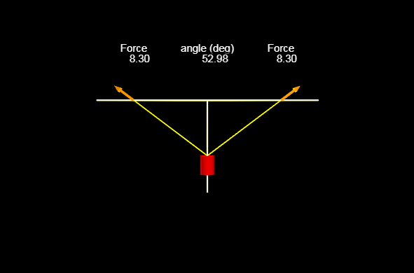
2 TwoForces 绘制效果

TwoForces.py绘制效果是一个动画，
这里展示其初始效果和结束效果。

初始效果

结束效果

3 代码逐行解析

posy=100;  Lcord=250  # basic height, cord length
Hweight=50;  W = 10   # cylinder height, weight

posy: 水平横线的高度
Lcord: 绳子长度
Hwight: 圆柱砝码的高度
W: 圆柱砝码的重量

alt=curve(pos=[(-300,posy,0),(300,posy,0)])
divi=curve(pos=[(0,-150,0),(0,posy,0)])
kilogr=cylinder(pos=vector(0,posy-Lcord,0),radius=20,axis=vector(0,-Hweight,0),
                color=color.red) # kg as a cylinder
cord1=cylinder(pos=vector(0,posy,0),axis=vector(0,-Lcord,0),color=color.yellow,
               radius=2)
cord2=cylinder(pos=vector(0,posy,0),axis=vector(0,-Lcord,0),color=color.yellow,
               radius=2)

arrow1=arrow(pos=vector(0,posy,0), color=color.orange) # Tension cord 1
arrow2=arrow(pos=vector(0,posy,0), color=color.orange) # Tension cord 2

alt: 在高为posy(100)的地方，绘制y轴左右各长300的水平线
divi: 在y轴上画一条竖直的线，从-150到高度为posy(100)。
kilogr: 创建一个红色圆柱体代表砝码，砝码半径为20，底部朝上，高度为Hweight(50)，底部中心在posy-Lcord的位置上
cord1
cord2

创建两条黄色绳子（没有半径），绳子尾在alt线中点，绳子长Lcord，头刚好拉住kilogr

由于没有半径，刚开始会被divi这条线挡住。

arrow1
arrow2

创建两个橘色箭头（弹簧拉钩），底部中心位置在alt线的中点，方向向上。

其长度可以展示力的大小

magF=W/2.0          # initial force of each student
v=2.0               # (m/s) velocity of each student
x1=0.0              # initial position student 1

计算与设置初始值

magF: 每个绳子上的力
v: 移动速度,箭头底部沿x轴的移动速度
x1: 箭头移动的距离（距离alt线的中点）

anglabel=label(pos=vector(0,240,0), text='angle (deg)',box=0)
angultext=label(pos=vector(20,210,0),box=0)
Flabel1=label(pos=vector(200,240,0), text='Force',box=0)
Ftext1=label(pos=vector(200,210,0),box=0)
Flabel2=label(pos=vector(-200,240,0), text='Force',box=0)
Ftext2=label(pos=vector(-200,210,0),box=0)

在指定的位置添加无框文本进行展示

在高度为240的地方，展示变量名字anglabel，Flabel1，Flabel2，

在高度为210的地方，展示变量值angultext，Ftext1，Ftext2，且后面还会不断更新这些变量值。

angultext展示的是绳子和竖直线divi形成的角度大小（角度制），

Ftext1，Ftext2展示两个绳子上的力的大小（两值相等）。

local_light(pos=vector(-10,0,20), color=color.yellow)   # light

添加一个局部点光源，效果不明显（基本没有）

for t in arange(0.,100.0,0.2):  
    rate(50)                  # slow motion

执行循环，从0到100间隔0.2取t值。
rate(50)设置循环每秒执行50次，每秒t增长50*0.2=10，相当于十倍速展示。

    x1=v*t                    # 1 to right, 2 to left
    theta=asin(x1/Lcord)      # angle cord
    poscil=posy-Lcord*cos(theta)  # cylinder height
    kilogr.pos=vector(0,poscil,0)     # y-position kilogram
    magF=W/(2.*cos(theta))      # Cord tension
    angle=180.*theta/pi

x1: 速度乘时间，得到位移
theta: 对边除斜边，得到sin，在通过asin算出绳子和竖直线的夹角值（弧度制）
poscil: 算出砝码上端中心的y轴位置
kilogr.pos: 更新砝码位置
magF: 算出绳子上的力
angle: 算出theta对应的角度制的值

    cord1.pos=vector(x1,posy,0)       # position cord end
    cord1.axis=vector(-Lcord*sin(theta),-Lcord*cos(theta),0)
    cord2.pos=vector(-x1,posy,0)            # position end cord
    cord2.axis=vector(Lcord*sin(theta),-Lcord*cos(theta),0)
    arrow1.pos=cord1.pos            # axis arrow 
    arrow1.axis=vector(8*magF*sin(theta),8*magF*cos(theta),0)
    arrow2.pos=cord2.pos
    arrow2.axis=vector(-8*magF*sin(theta),8*magF*cos(theta),0)

重新设置两根绳子的位置pos(更新水平坐标)和方向axis。

重新设置两个箭头的位置pos(和绳子pos相同)和方向axis，方向向量的数值（箭头长）能展示力的大小变化。

    angultext.text='%4.2f'%angle
    force=magF
    Ftext1.text='%8.2f'%force     # Tension
    Ftext2.text='%8.2f'%force

更新文本标签

'%4.2f' 字符宽度设置为4，保留2位有效数字
'%8.2f' 字符宽度设置为8，保留2位有效数字

5 - Vpython 三解读

1 `cone`

doc: https://www.glowscript.org/docs/VPythonDocs/cone.html

建立一个圆锥体。

代码示例

cone(pos=vector(5,2,0), axis=vector(12,0,0), radius=1)

参数官方示意图

2 `box`

doc: https://www.glowscript.org/docs/VPythonDocs/box.html

建立一个立方体。
代码示例

mybox = box(pos=vector(x0,y0,z0), length=L, height=H, width=W)
mybox = box(pos=vector(x0,y0,z0), axis=vector(a,b,c), size=vector(L,H,W))
mybox = box(pos=vector(x0,y0,z0), axis=vector(a,b,c), length=L, height=H, width=W, up=vector(q,r,s))

pos: the center of the box
axis: (a, b, c)
size: (L, H, W), default is vector(1,1,1)

说明，不指定L的话，axis的a就是L，指定了L的话，axis只约束L的方向。(The axis attribute gives a direction for the length of the box)

up: (q,r,s)

the width of the box will lie in a plane perpendicular to the (q,r,s) vector,
and the height of the box will be perpendicular to the width and to the (a,b,c) vector.

方框的宽度将垂直于(q,r,s)矢量，方框的高度将垂直于宽度和(a,b,c)矢量。

参数官方示意图

3 textures

doc: https://www.glowscript.org/docs/VPythonDocs/textures.html
textures是Vpython7的新特性，通过texture这个参数名来指定。在Classic Vpython(Vpython 6)中，原本叫做materials，通过material参数名来指定。

设置对象的纹理（贴图）。

简单指定方法如下

box(texture=textures.stucco)

stucco是指定其为粉饰灰泥纹理。

纹理支持的所有值和对应的效果如下

{
    "flower": "花", 
    "granite": "花岗岩", 
    "gravel": "砾石", 
    "earth": "地球", 
    "metal": "金属", 
    "rock": "岩石", 
    "rough": "粗糙的", 
    "rug": "小地毯", 
    "stones": "石头", 
    "stucco": "灰泥", 
    "wood": "木材", 
    "wood_old": "老木头"
}

以1.10 的 SlidingBox.py为例，展示下有纹理和无纹理的效果区别

有纹理的示例代码如下。

from vpython import *

Hsupport=30;  d=100                # height, distance supports
Lbeam=500; Wbeam=80;  thickness=10 # beam dimensions
Lbox=60; Wbox=60; Hbox=60  # Box Dimensions

# Graphics
scene=canvas(width=750, height=500,range=300)
scene.forward=vector(0.5,-0.2,-1)  # to change point of view

beam=box(pos=vector(0,Hsupport+thickness/2,0),color=color.orange, length=Lbeam,width=Wbeam,height=thickness,texture=textures.wood)
cube=box(pos=vector(-d,Hsupport+Hbox/2+thickness,0),length=Lbox, width=Wbox,height=Hbox,texture=textures.rock)

有纹理的效果如下图

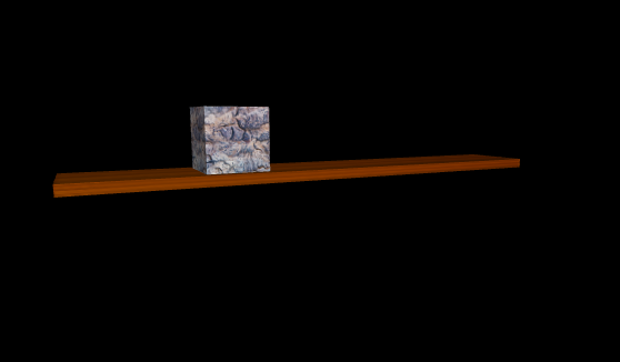
无纹理的效果如下图(删除指定纹理参数的代码)

6 - 1.10 SlidingBox.py

1 代码展示

from vpython import *

Hsupport=30;  d=100                # height, distance supports
Lbeam=500; Wbeam=80;  thickness=10 # beam dimensions     
W =200;  WeightBox=400             # weight of table,box 
Lbox=60; Wbox=60; Hbox=60 # Box Dimensions

# Graphics
scene=canvas(width=750, height=500,range=300)
scene.forward=vector(0.5,-0.2,-1)  # to change point of view
support1=cone(pos=vector(-d,0,0),axis=vector(0,Hsupport,0),color=color.yellow,
              radius=20)
support2=cone(pos=vector(d,0,0),axis=vector(0,Hsupport,0),color=color.yellow,
              radius=20)
beam=box(pos=vector(0,Hsupport+thickness/2,0),color=color.orange, length=Lbeam,width=Wbeam,height=thickness,texture=textures.wood)
cube=box(pos=vector(-d,Hsupport+Hbox/2+thickness,0),length=Lbox, width=Wbox,height=Hbox,texture=textures.rock)
piso=curve(pos=[(-300,0,0),(300,0,0)],color=color.green, radius=1)
arrowcube=arrow(color=color.orange,axis=vector(0,-0.15*Wbox,0)) # scale 
arrowbeam=arrow(color=color.orange,axis=vector(0,-0.15*W,0))
arrowbeam.pos=vector(0,Hsupport+thickness/2,0) 

v=4.0                           # box speed
x=-d                            # box initial position
Mg=WeightBox+W                  # weight box+beam
Fl=(2*Wbox+W)/2.0               
arrowFl=arrow(color=color.red,pos=vector(-d,Hsupport+thickness/2,0), axis=vector(0,0.15*Fl,0))
Fr=Mg-Fl                        # right force
arrowFr=arrow(color=color.red,pos=vector(d,Hsupport+thickness/2,0), axis=vector(0,0.15*Fr,0))
anglabel=label(pos=vector(-100,150,0), text='Fl=',box=0)   
Ftext1=label(pos=vector(-50,153,0),box=0)                  
anglabel2=label(pos=vector(100,150,0), text='Fr=',box=0)
Ftext2=label(pos=vector(150,153,0),box=0)
rate(4)                         # to slow motion

for t in arange(0.0,65.0,0.5):                           
    rate(10)                                         
    x=-d+v*t
    cube.pos=vector(x, Hsupport+Hbox/2+10,0) # position cube
    arrowcube.pos=vector(x,Hsupport+5,0)
    if Fl>0:                                  
        Fl=(d*Mg-x*WeightBox)/(2.0*d)   
        Fr=Mg-Fl                              
        cube.pos=vector(x, Hsupport+Hbox/2+10,0)   
        arrowcube.pos=vector(x,Hsupport+thickness/2,0)  
        arrowFl.axis=vector(0,0.15*Fl,0)          
        arrowFr.axis=vector(0,0.15*Fr,0)         
        Ftext1.text='%8.2f'%Fl                   # Left force value
        Ftext2.text='%8.2f'%Fr                   # Right force value
    elif Fl==0:                                   
         x=300
         beam.rotate(angle=-0.2,axis=vector(0,0,1),
          origin=vector(d,Hsupport+thickness/2,0))
         cube.pos=vector(300,Hsupport,0)
         arrowcube.pos=vector(300,0,0)
         break
    
rate(5) 
arrowFl.axis=vector(0,0.15*0.5*(W),0)  # return beam
arrowFr.axis=arrowFl.axis
beam.rotate(angle=0.2,axis=vector(0,0,1),origin=vector(d,Hsupport+thickness/2,0))
Fl=100.0
Ftext1.text='%8.2f'%Fl
Ftext2.text='%8.2f'%Fl

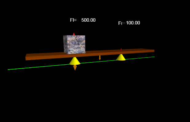
2 运行效果

这个代码运行效果是一个动画：
立方体在横木上从左往右移动，移动到右边的锥子右边后，掉落到水平面。

这里展示其三阶段的效果。

初始效果

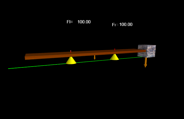
中间效果

最终效果

3 逐行解读

Hsupport=30;  d=100                # height, distance supports
Lbeam=500; Wbeam=80;  thickness=10 # beam dimensions     
W =200;  WeightBox=400             # weight of table,box 
Lbox=60; Wbox=60; Hbox=60 # Box Dimensions

Hsupport: 黄色圆锥体（支撑）的高度
d: 黄色圆锥体（支撑）和水平中心的举例，x轴的偏移量
Lbeam, Wbeam, thickness: 横木梁的长，宽，高（厚度）
W: 横木梁的重量
WeightBox: 立方体（箱子）的重量
Lbox, Wbox, Hbox: 立方体（箱子）的长，宽，高（厚度）

scene=canvas(width=750, height=500,range=300)
scene.forward=vector(0.5,-0.2,-1)  # to change point of view

新建画板为场景，
更改场景相机的方向(forward)

forward: Vector pointing in the same direction as the camera looks (that is, from the current camera location, given by scene.camera.pos, toward scene.center). When forward is changed, either by program or by the user using the mouse to rotate the camera position, the camera position changes to continue looking at center. Default vector(0,0,-1). Its magnitude is not significant.

可看前文3 - Vpython 再解读的1 canvas的示意图。

support1=cone(pos=vector(-d,0,0),axis=vector(0,Hsupport,0),color=color.yellow,
              radius=20)
support2=cone(pos=vector(d,0,0),axis=vector(0,Hsupport,0),color=color.yellow,
              radius=20)
beam=box(pos=vector(0,Hsupport+thickness/2,0),color=color.orange, length=Lbeam,width=Wbeam,height=thickness,texture=textures.wood)
cube=box(pos=vector(-d,Hsupport+Hbox/2+thickness,0),length=Lbox, width=Wbox,height=Hbox,texture=textures.rock)
piso=curve(pos=[(-300,0,0),(300,0,0)],color=color.green, radius=1)

# Origin code in Book use WBox, I think it should be wrong
arrowcube=arrow(color=color.orange,axis=vector(0,-0.15*WeightBox,0)) # scale 
arrowbeam=arrow(color=color.orange,axis=vector(0,-0.15*W,0))
arrowbeam.pos=vector(0,Hsupport+thickness/2,0)

support1, support2: 两个黄色圆锥体，支撑物
beam: 橘色横木梁，贴图为木头贴图
cube: 立方体箱子，题图为岩石贴图
piso: 地板上的一条绿色线，和x轴平行。
arrowcube: 橘色箭头，示意立方体箱子受到的重力，
arrowbeam: 橘色箭头，示意横木梁的重力，
更改其y轴位置为横木梁上面中心。

v=4.0                           # box speed
x=-d                            # box initial position
Mg=WeightBox+W                  # weight box+beam
Fl=(2*WeightBox+W)/2.0          # Origin code in Book that should be wrong: Fl=(2*WBox+W)/2.0  
arrowFl=arrow(color=color.red,pos=vector(-d,Hsupport+thickness/2,0), axis=vector(0,0.15*Fl,0))
Fr=Mg-Fl                            # right force
arrowFr=arrow(color=color.red,pos=vector(d,Hsupport+thickness/2,0), axis=vector(0,0.15*Fr,0))

v: 立方体箱子的移动速度
x: 立方体x轴坐标，初始时应该为-d
Mg: 立方体箱子和横木梁的重力
Fl, Fr: 左边, 右边支撑体圆锥分到的力
arrowFl, arrowFr: 左边, 右边的箭头，用于展示左右边圆锥体的支撑力。

anglabel=label(pos=vector(-100,150,0), text='Fl=',box=0)   
Ftext1=label(pos=vector(-50,153,0),box=0)                  
anglabel2=label(pos=vector(100,150,0), text='Fr=',box=0)
Ftext2=label(pos=vector(150,153,0),box=0)
rate(4)                         # to slow motion

anglabel, anglabel2: 展示左右两边力的名字
Ftext1, Ftext2: 展示左右两边力的值

box = 0 表示无框

rate(4) 1/4秒后执行下一句

for t in arange(0.0,65.0,0.5):                           
    rate(10)                                         
    x=-d+v*t
    cube.pos=vector(x, Hsupport+Hbox/2+10,0) # position cube
    arrowcube.pos=vector(x,Hsupport+5,0)

执行循环，从0到65间隔0.5取t值。
设置循环每秒执行10次，每秒t增长 10*0.5=5 ，相当于5倍速展示。
根据速度公式计算位移
重新设置立方体箱子的位置，只修改了x。
10是指thickness（横木梁的高度即厚度），这里写死数值不好，更应该写成thickness。
更改箭头arrowcube的位置，该箭头示意立方体箱子的重力。

    if Fl>0:                                  
        Fl=(d*Mg-x*WeightBox)/(2.0*d)   
        Fr=Mg-Fl                              
        cube.pos=vector(x, Hsupport+Hbox/2+10,0)   
        arrowcube.pos=vector(x,Hsupport+thickness/2,0)  
        arrowFl.axis=vector(0,0.15*Fl,0)          
        arrowFr.axis=vector(0,0.15*Fr,0)         
        Ftext1.text='%8.2f'%Fl                   # Left force value
        Ftext2.text='%8.2f'%Fr

Fl>0: 代表左边圆锥支撑还受到压力，说明此事立方体箱子还在两个圆锥支撑之间。
计算左右两边圆锥收到的压力（数值上也等于其支持力）
Fl是根据杠杆原理的公式计算的（有一点不太相同）
cube.pos, arrowcube.pos: 这两行代码和上面相同，是多余的。
更新左右两边示意圆锥支撑体支持力的的红色箭头的长度
更新左右两边文本上展示的力的值。
'%8.2f': 占位符总长度为8位，保留两位有效数字（保留两位小数）。

    elif Fl==0:                                   
         x=300
         beam.rotate(angle=-0.2,axis=vector(0,0,1),
          origin=vector(d,Hsupport+thickness/2,0))
         cube.pos=vector(300,Hsupport,0)
         arrowcube.pos=vector(300,0,0)
         break

Fl==0: 左边圆锥支撑无压力的话，说明左边已经翘起来了，立方体箱子将从右边滑下。
x=300: 箱子直接滑到横木梁最右边
横木梁会以右边圆锥为支点，翘起来一点
更新箱子位置
更新箱子的重力示意箭头位子
break: 退出for循环

rate(5) 
arrowFl.axis=vector(0,0.15*0.5*(W),0)  # return beam
arrowFr.axis=arrowFl.axis
beam.rotate(angle=0.2,axis=vector(0,0,1),origin=vector(d,Hsupport+thickness/2,0))
Fl=100.0
Ftext1.text='%8.2f'%Fl
Ftext2.text='%8.2f'%Fl

rate(5): 1/5秒后执行后面的代码
arrowFl, arrowFr: 更新左右两边示意圆锥支撑体支持力的的红色箭头的长度
横木梁归位
更新左边圆锥支持力的大小
更新左右两边文本上展示的力的值。

7 - 1.11 CentralValue.py

1 代码展示

import random
import numpy as np, matplotlib.pyplot as plt

N = 1000; NR = 10000   #  Sum N variables, distribution of sums 
SumList = [] # empty list

def SumRandoms():  # Sum N randoms in [0,1]
    sum = 0.0
    for i in range(0,N):  sum = sum + random.random() 
    return sum                    
    
def normal_dist_param():
    add = sum2 =0 
    for i in range(0,NR):  add = add + SumList[i]
    mu = add/NR               # Average distribution
    for i in range(0,NR): sum2 = sum2 + (SumList[i]-mu)**2
    sigma = np.sqrt(sum2/NR)
    return mu,sigma    

for i in range(0,NR):
    dist =SumRandoms()      
    SumList.append(dist)           # Fill list with NR sums

plt.hist(SumList, bins=100, density=True) # True: normalize
mu, sigma = normal_dist_param()            
x = np.arange(450,550)
rho = np.exp(-(x-mu)**2/(2*sigma**2))/(np.sqrt(2*np.pi*sigma**2)) 

plt.plot( x,rho, 'g-', linewidth=3.0)         # Normal distrib
plt.xlabel('Random Number x 1000')
plt.ylabel('Average of Random Numbers')
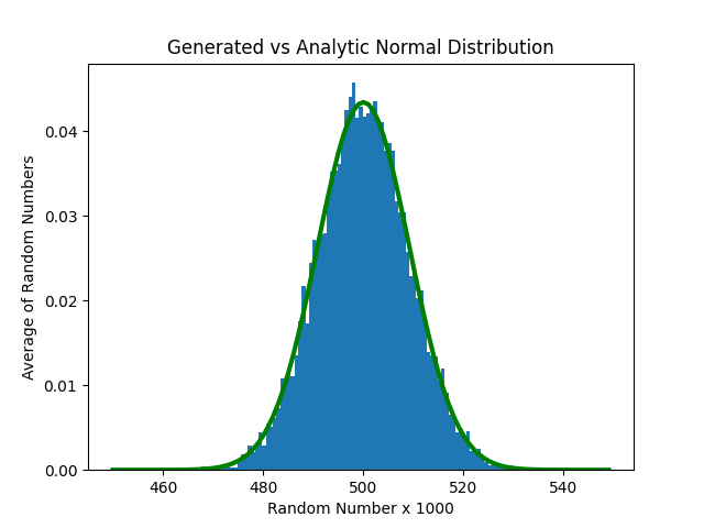
plt.title('Generated vs Analytic Normal Distribution')
plt.show()

2 运行效果

3 plt.hist

doc: matplotlib.pyplot.hist

简易写法为

plt.hist(x, **kwargs)

计算并绘制x的直方图。

可通过kwargs来进行一些设置。
用到的

bins: 可选参数，可为整数、序列或字符串。
如果是整数，则定义范围内等宽的柱的数量。
density: 可选参数，布尔值(boolean)。
是否按密度probability density绘制

已经遗弃的参数（书上用过）

normed: 该参数已被density替换。

4 逐行解析

def SumRandoms():  # Sum N randoms in [0,1]
    sum = 0.0
    for i in range(0, N):  sum = sum + random.random()
    return sum

计算[0,1]中N个随机数之和并返回
返回值是一个[0,N]之间的值

for i in range(0,NR):
    dist =SumRandoms()      
    SumList.append(dist)           # Fill list with NR sums

循环NR次，在SumList列表中添加NR个SumRandoms()的值

plt.hist(SumList, bins=100, density=True) # True: normalize

绘制SumList的分布直方图，按密度绘制，分为100段。

def normal_dist_param():
    add = sum2 =0
    for i in range(0,NR):  add = add + SumList[i]
    mu = add/NR               # Average distribution
    for i in range(0,NR): sum2 = sum2 + (SumList[i]-mu)**2
    sigma = np.sqrt(sum2/NR)
    return mu,sigma  

mu, sigma = normal_dist_param()

计算SumList的平均值mu和标准差sigma

x = np.arange(450,550)
rho = np.exp(-(x-mu)**2/(2*sigma**2))/(np.sqrt(2*np.pi*sigma**2))

np.arange(450,550)没有写步长（间隔值），说明使用默认值1。
x为一个450到550之间隔1取值组成的数组。

rho这里用到了正态分布公式

[frac{e^{-frac{(x-mu)^2}{2 sigma^2}}}{sqrt{2pi sigma^2}}, 其中平均值mu对应代码中的mu，标准差sigma对应代码中的sigma ]

plt.plot( x,rho, 'g-', linewidth=3.0)         # Normal distrib

绘制刚才的符合正态分布公式的x和xho，
用绿色曲线绘制。

相关阅读:
InnoDB的数据页结构
 InnoDB的行溢出数据,Char的行结构存储
 InnoDB的行记录格式, Compact, Redundant, Compressed, Dynamic
python py_innodb_page_info.py -v /usr/local/var/mysql/ibdata1
InnoDB的表类型,逻辑存储结构,物理存储结构
 InnoDB存储引擎的表空间文件,重做日志文件
 MYSQL数据库的套接字文件,pid文件,表结构文件
 MYSQL数据库的日志文件
 MYSQL数据库的参数文件
 InnoDB的启动,关闭,恢复
原文地址：https://www.cnblogs.com/BigShuang/p/14536561.html

python一对一教程：Computational Problems for Physics chapter 1-B Code Listings 1.7

1 - 1.7 PondMatPlot.py

1 subplots

2 .axes.Axes 的方法

3 PondMatPlot 绘制效果

4 PondMatPlot 逐行解析

2 - 1.8 PondMatPlot.py

1 PondMatPlot绘制效果

2 fig.add_subplot

3 代码逐行解析

3 - Vpython 再解读

1 canvas

2 curve

3 cylinder

4 arrow

5 label

6 local_light

7 rate

4 - 1.9 TwoForces.py

1 为Vpython7更新代码语法

2 TwoForces 绘制效果

3 代码逐行解析

5 - Vpython 三解读

1 cone

2 box

3 textures

6 - 1.10 SlidingBox.py

1 代码展示

2 运行效果

3 逐行解读

7 - 1.11 CentralValue.py

1 代码展示

2 运行效果

3 plt.hist

4 逐行解析

2 `.axes.Axes` 的方法

1 `canvas`

2 `curve`

3 `cylinder`

4 `arrow`

5 `label`

6 `local_light`

7 `rate`

1 `cone`

2 `box`