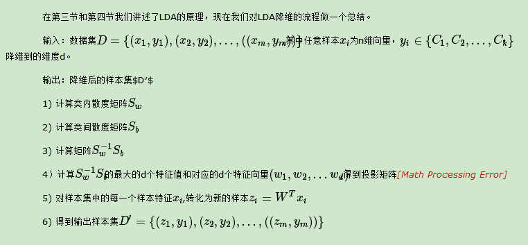
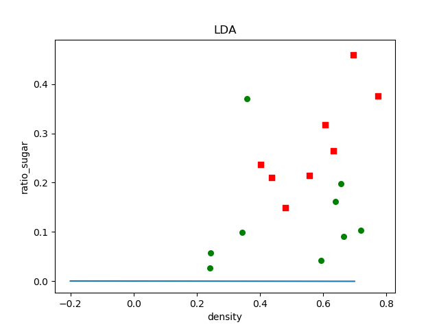
一、LDA线性判决分类
总之求解
1、计算每类均值u0,u1为向量
2、计算Sw
3
  w=(u0 - u1) * (mat(sw).I)
以机器学习西瓜数据3.0为例
from numpy import *
import numpy as np
import matplotlib.pyplot as plt
import math
# pandas 模块可以将读取到的表格型数据,进行数据列,行操作
import pandas as pd
# 也可以读取.txt格式,仍用read_csv
data=pd.read_csv("watermelon_3a.csv")
#获取的用列表保存
def calculate_w():
 df1= data[data.label==1]
 df2= data[data.label==0]
 #获取每个标签对应的数据值.values
 X0=df1.values[:,1:3]
 X1=df2.values[:,1:3]
 #计算每类均值u0,u1为向量,mean只计算向量,不能矩阵
 u0= array ([mean(X0[:,0]),mean(X0[:,1])])
 u1= array ([mean(X1[:,0]),mean(X1[:,1])])
 #产生全为u0和u1矩阵
 m1 = shape(X1)[0]
#shape[1] 为第二维的长度,shape[0] 为第一维的长度,矩阵的行数
#mat   函数将数据类型为数组的转化为矩阵形式,进行线代操作
 sw = zeros(shape=(2, 2))
 for i in range (m1):
    xsmean=mat(X1[i,:]-u1)
    sw += xsmean.transpose() * xsmean
 m0 = shape(X0)[0]
 for i in range (m0):
    xsmean=mat(X0[i,:]-u0)
    sw += xsmean.transpose() * xsmean
 w = (u0 - u1) * (mat(sw).I)
 return w

def plot(w):
 dataMat=array(data[['density','ratio_sugar']].values[:,:])
 labelMat = mat(data['label'].values[:]).transpose()
 print(labelMat)
 m=shape(dataMat)[0]
 xcord1 = []
 ycord1 = []
 xcord2 = []
 ycord2 = []
 for i in range(m):
        if labelMat[i] == 1:
            xcord1.append(dataMat[i, 0])
            ycord1.append(dataMat[i, 1])
        else:
            xcord2.append(dataMat[i, 0])
            ycord2.append(dataMat[i, 1])
 plt.figure(1)
 # 将画面分割成1行一列第1个图
 ax = plt.subplot(111)
 ax.scatter(xcord1, ycord1, s=30, c='red', marker='s')
 ax.scatter(xcord2, ycord2, s=30, c='green')
 x = arange(-0.2, 0.8, 0.1)
 #a=0.00066,b=0.9直线的斜率为-a/b,直线方程为kx
 a=w[0,0]
 b=w[0,1]
 u=(-w[0, 0] * x) / w[0, 1]
 y = array(u)
 print(shape(x))
 print(shape(y))
 plt.sca(ax)
 plt.plot(x, y)  # gradAscent
 plt.xlabel('density')
 plt.ylabel('ratio_sugar')
 plt.title('LDA')
 plt.show()

w=calculate_w()
print(w)
plot(w)
注意:求解出来的w=[w0,w1]垂直于我们的直线,所以斜率-w0/w1;实现的结果如下
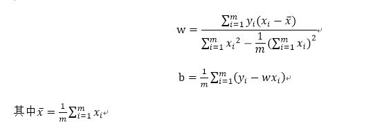
二、logistic回归
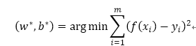
1、几何几率回归
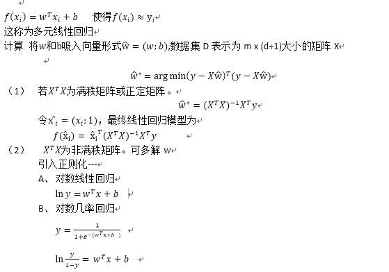
f(xi)=w xi +b;使得f(xi)≈yi
输入属性的数目只有一个
样本若有d个属性描述
在次程序中采用梯度上升和随机梯度上升法
主要区别在于
1、alpha的变化所有
2、批量梯度上升,每次进行一次迭代更新就计算所有的样本;随机样本梯度上升:根据样本的数量进行迭代,每次计算一个样本进行一次更新
(梯度上升)
step1:获取数据,X为m x (d+1)矩阵,权值初始化w为(d+1)x 1;
step2: 计算预测值输出值h=sigmoid(X*w)
step3:计算误差 error=label-h
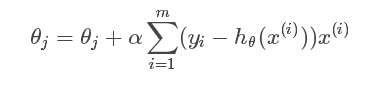
step4: 更新公式如下
step5:画出plot(w)
注意直线w=[w0,w1,w2];前两项为-w0/w1仍然为直线的斜率,我感觉w2直接就是之前的b,但是在实际中用-w2/w1?????目前还不知道为什么?谁看明白可以告诉我,谢谢
from numpy import *
import numpy as np
import matplotlib.pyplot as plt
import pandas as pd
#利用几何几率回归将西瓜数据进行分类,并用梯度上升和随机梯度上升求解w,b
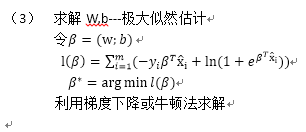
#最小化损失函数-梯度下降;最大化极大似然函数--梯度上升法
# 读入csv文件数据
data = pd.read_csv('watermelon_3a.csv')
m, n = shape(data)
data['norm'] = ones((m, 1))
print(data)
#step1,先求出X为 m x(d+1)=17x3,第三个元素直接赋值为1,不需要在values[:,:,:]
#dataLabel为实际值{0,1}
dataMat=array(data[['density','ratio_sugar','norm']].values[:,:])
dataLabel=mat(data[['label']].values[:]).transpose()
def GradAscend():
#对权值初始化,全一
itermax=300
n=shape((dataMat))[1]
a=0.1
w=array(ones((n,1)))
for i in range (itermax):
u=dot(dataMat,w)
h=sigmoid(u)
erro=dataLabel.transpose()-h
w= w +a*( dataMat .transpose() *erro)
return w
def sigmoid(x):
return (1/(1+exp(-x)))
def plot(w):
dataMat1=array(data[['density','ratio_sugar']].values[:,:])
dataLabel1=mat(data[['label']].values[:])
xcard1=[]
ycard1=[]
xcard2=[]
ycard2=[]
m=shape(dataMat1)[0]
for i in range(m):
if (dataLabel1[i]==1):
xcard1.append(dataMat1[i,0])
ycard1.append(dataMat1[i,1])
else:
xcard2.append(dataMat1[i,0])
ycard2.append(dataMat1[i,1])
plt.figure(1)
ax=plt.subplot(111)
ax.scatter(xcard1, ycard1, s=30, c='red', marker='s')
ax.scatter(xcard2, ycard2, s=30, c='green')
x = arange(0.2, 0.8, 0.1)
W1=mat(w).transpose()
#y=array(((-W1[0, 2] - W1[0, 0]* x) /W1[0,1]))
y = array(((-W1[0, 2] - W1[0, 0] * x) / W1[0, 1]))
shape(x)
shape(y)
plt.sca(ax)
plt.plot(x, y) # ramdomgradAscent
# plt.plot(x,y[0]) #gradAscent
plt.xlabel('density')
plt.ylabel('ratio_sugar')
# plt.title('gradAscent logistic regression')
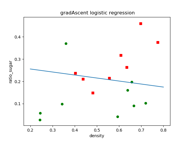
plt.title(' gradAscent logistic regression')
plt.show()
w=GradAscend()
print(w)
plot(w)
结果
w=
[[ 1.20808298]
[ 8.92638039]
[-2.52407404]]
划分结果
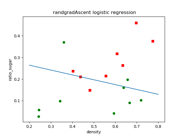
(2)随机梯度下降
from numpy import *
import numpy as np
import matplotlib.pyplot as plt
import pandas as pd

# 利用几何几率回归将西瓜数据进行分类,并用梯度上升和随机梯度上升求解w,b
# 最小化损失函数-梯度下降;最大化极大似然函数--梯度上升法

# 读入csv文件数据
data = pd.read_csv('watermelon_3a.csv')
m, n = shape(data)
data['norm'] = ones((m, 1))
print(data)
# step1,先求出X为 m x(d+1)=17x3,第三个元素直接赋值为1,不需要在values[:,:,:]
# dataLabel为实际值{0,1}
dataMat = array(data[['density', 'ratio_sugar', 'norm']].values[:, :])
dataLabel = mat(data[['label']].values[:]).transpose()


def sigmoid(x):
    return (1 / (1 + exp(-x)))

def randomgradAscent(dataMat,dataLabel):
  m, n = shape(dataMat)
  numIter=50
  w = ones(n)

  for j in range(numIter):
     dataIndex =list( range(m))
     for i in range(m):
          alpha = 4.0 / (1.0 + j + i) + 0.2
          randIndex_Index = int(random.uniform(0, len(dataIndex)))
          randIndex = dataIndex[randIndex_Index]
          h = sigmoid(sum(dot(dataMat[randIndex], w)))
          error = (dataLabel[0,randIndex] - h)
          w = w + alpha * error * (dataMat[randIndex].transpose())
          del (dataIndex[randIndex_Index])

  return w


def plot(w):
    dataMat1 = array(data[['density', 'ratio_sugar']].values[:, :])
    dataLabel1 = mat(data[['label']].values[:])
    xcard1 = []
    ycard1 = []
    xcard2 = []
    ycard2 = []
    m = shape(dataMat1)[0]
    for i in range(m):
        if (dataLabel1[i] == 1):
            xcard1.append(dataMat1[i, 0])
            ycard1.append(dataMat1[i, 1])
        else:
            xcard2.append(dataMat1[i, 0])
            ycard2.append(dataMat1[i, 1])
    plt.figure(1)
    ax = plt.subplot(111)
    ax.scatter(xcard1, ycard1, s=30, c='red', marker='s')
    ax.scatter(xcard2, ycard2, s=30, c='green')
    x = arange(0.2, 0.8, 0.1)
    #W1 = mat(w).transpose()
    # y=array(((-W1[0, 2] - W1[0, 0]* x) /W1[0,1]))
    y = array(((-w[2] - w[0] * x) / w[1]))
    print
    shape(x)
    print
    shape(y)
    plt.sca(ax)
    plt.plot(x, y)  # ramdomgradAscent
    # plt.plot(x,y[0])   #gradAscent
    plt.xlabel('density')
    plt.ylabel('ratio_sugar')
    # plt.title('gradAscent logistic regression')
    plt.title(' randgradAscent logistic regression')
    plt.show()
w =randomgradAscent(dataMat,dataLabel)
print(w)
plot(w)
w=[ 1.59035763 7.07872188 -2.18857215]